
Introduction to Turbulent Flow
Enroll to start learning
You’ve not yet enrolled in this course. Please enroll for free to listen to audio lessons, classroom podcasts and take practice test.
Interactive Audio Lesson
Listen to a student-teacher conversation explaining the topic in a relatable way.
Shear Stress and Velocity Profile
🔒 Unlock Audio Lesson
Sign up and enroll to listen to this audio lesson

Let's start with the concept of shear stress in turbulent flow. When the flow is turbulent, the shear stress at the wall is constant and denoted as τ₀. Why is that important?

It's important because it simplifies our calculations, right?
Exactly! When we assume τ = τ₀, we can express the velocity gradient du/dy in simpler terms. Can anyone recall the relationship we get with the small value of y?

Is it related to κ and y, where du/dy becomes 1/κ * y?
Very close! It essentially helps us derive the logarithmic velocity profile, which is crucial in turbulent flow. Remembering that τ₀ represents wall shear stress can serve as a mnemonic for understanding turbulence.

So, the turbulent flow profile is different from laminar flow, which was parabolic, right?
Correct! Turbulent flow has a fuller velocity profile due to fluctuations. Any thoughts on how this affects real-world applications?

It likely affects anything from pipe design to understanding natural river flows.
Great observations! So far, we've established that τ₀ is pivotal in analyzing turbulent flow's properties.
Logarithmic Velocity Profile
🔒 Unlock Audio Lesson
Sign up and enroll to listen to this audio lesson

Now that we understand shear stress, let’s explore the derivation of the logarithmic velocity profile. Using boundary conditions, how can we express u at y = R?
u at y = R would equal u_max, right?
Exactly! Substituting this into our equation allows us to isolate C. What do we get?
C = u_max - u_* / κ ln R?
Correct! So when we manipulate this, we derive the velocity defect law. Does anyone recall what that is?
It shows the difference between maximum velocity and actual velocity in turbulent flow?
That’s right! It's significant in designing more efficient systems in fluid transport. Can someone explain how the shape differs from laminar profiles?
The turbulent profile is fuller compared to the parabolic shape of laminar flow.
Exactly! Understanding these profiles allows engineers to predict flow behavior.
Boundary Layers and Their Classifications
🔒 Unlock Audio Lesson
Sign up and enroll to listen to this audio lesson
Let's dive into the concept of boundary layers in turbulent flows. What layers can we identify?
Viscous sublayer, buffer layer, overlap layer, and turbulent layer.
Excellent! The viscous sublayer is where viscous effects are dominant. Can someone explain what happens in the buffer layer?
The turbulent effects start becoming significant, but the viscous effects still play a role.
Correct! Now, what terminology do we use to classify boundary types based on surface roughness?
Smooth boundaries and rough boundaries based on the height of surface irregularities.
Exactly! Remember, k represents the height of surface irregularities. If k is much larger than the viscous sublayer's thickness, we have a rough boundary. What determines transitional boundaries?
If the ratio k/δ is between 0.25 and 6, the boundary is transitional.
Correct! Understanding these characteristics helps engineers design for different flow scenarios.
Practical Implications of Turbulent Flow
🔒 Unlock Audio Lesson
Sign up and enroll to listen to this audio lesson
Now that we have the theory down, let’s discuss real-world applications. Why do we care about turbulent flow in pipe systems?
It affects pressure drop and energy loss in pumping systems.
Absolutely! Let's consider a practical example: If a pipe has a diameter of 10 cm, how might you calculate shear stress?
We could use τ₀ = ρu*² or apply boundary conditions to find relationships.
Good point! Remember, turbulent flow leads to different pressure measurements than laminar. What insights does that give us?
Engineers must account for these differences when designing systems to prevent inefficiencies.
Exactly! Understanding turbulent flow guides solutions to optimize performance in various engineering applications.
Introduction & Overview
Read summaries of the section's main ideas at different levels of detail.
Quick Overview
Standard
The section outlines the relationship between shear stress and velocity in turbulent flow. It provides equations derived from Prandtl's mixing length theory and illustrates the differences between laminar and turbulent velocity profiles. Additionally, it introduces concepts of boundary layers and the classification of smooth and rough boundaries.
Detailed
Introduction to Turbulent Flow
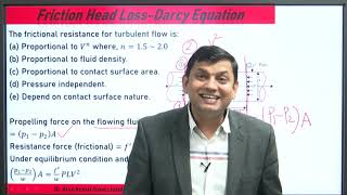
Turbulent flow is characterized by chaotic fluctuations in velocity and pressure. In this section, we explore essential equations governing turbulent flow, particularly focusing on shear stress and the velocity profile. The discussion begins with the application of Equation 14 and how it relates to wall shear stress, denoted by τ₀, which remains constant at the pipe wall. As y approaches zero, we can simplify our equations to derive critical relationships.
Key Points:
- Shear Stress and Velocity: Under small values of y, τ can be approximated as τ₀, leading to simplified expressions for the velocity gradient du/dy in relation to κ and y.
- Logarithmic Velocity Profile: Using boundary conditions, we derive a logarithmic velocity profile for turbulent flow, showing a distinct contrast to the parabolic velocity profile seen in laminar flow.
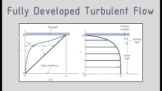
- Boundary Layers: We discuss the existence of various layers in turbulent flow: the viscous sublayer, buffer layer, overlap layer, and turbulent layer, each characterized by different effects of viscosity and turbulence.
- Roughness and Boundary Classification: Introduced by Nikuradse, we classify boundaries as smooth or rough based on the ratio of surface irregularities to the thickness of the viscous sublayer. Key thresholds are explored, along with real-world implications on boundary layer flow.
Understanding these principles is crucial for engineers and scientists working with fluid dynamics and flow systems.
Youtube Videos


Audio Book
Dive deep into the subject with an immersive audiobook experience.
Understanding Shear Stress in Turbulent Flow
Chapter 1 of 6
🔒 Unlock Audio Chapter
Sign up and enroll to access the full audio experience
Chapter Content
So, if we use equation 14 in equation 15, what was equation 14? l m was kappa into y, this was what we said in equation number 14. So, we can simply write...can be assumed to be a constant. So, at the wall the shear stress is assumed to be constant and equal to tau not.
Detailed Explanation
To understand turbulent flow, it's important to recognize how shear stress behaves in these conditions. In turbulent flow, shear stress at the wall (tau not) is considered constant, which allows simplifications in calculations. Here, the symbol 'kappa' relates to the mixing length, which quantifies how much mixing occurs at different distances from the pipe wall. This is crucial in deriving other equations relevant to turbulent flow dynamics.
Examples & Analogies
Think of a river with varying flow speeds. Near the riverbed (like the wall of a pipe), the water moves much slower due to friction (analogous to shear stress), while the top layers of water flow more freely. The idea of constant shear stress helps simplify how we understand the interaction between these layers.
Velocity Gradient and Shear Velocity
Chapter 2 of 6
🔒 Unlock Audio Chapter
Sign up and enroll to access the full audio experience
Chapter Content
And therefore, what we can say, if we substitute tau is equal to tau not in equation 16, we can obtain...under root tau / rho is rho u *.
Detailed Explanation
By substituting shear stress (tau) with its constant value at the wall (tau not) in our equations, we derive a relationship that connects the velocity gradient (du/dy) to shear velocity (u*). This relationship is fundamental in fluid dynamics as it allows us to relate shear stress to flow behavior. The term 'under root tau / rho' relates to the concept of shear velocity, which helps in determining the flow characteristics of turbulent fluid.
Examples & Analogies
Imagine a sliding box on a surface. The speed at which the box accelerates depends on the force applied (analogous to shear stress) and the weight of the box (analogous to density). By understanding this relationship, we can predict how quickly the box will slide, just like shear velocity helps us predict the flow rate in turbulent conditions.
Integration and Boundary Conditions
Chapter 3 of 6
🔒 Unlock Audio Chapter
Sign up and enroll to access the full audio experience
Chapter Content
If you integrate the equation number 17, so, what we can get is...C will be u max minus u * / kappa ln R.
Detailed Explanation
After deriving the equations, the next step is to integrate them to find the velocity profile of the turbulent flow. A key boundary condition used is that at the maximum radius (R) of the pipe, the velocity is at its maximum (u max). By substituting this boundary condition into our equations, we arrive at a formula that allows us to express the velocity at any point within the pipe's radius based on its distance from the wall.
Examples & Analogies
Think of this as mapping a hill. At the peak of the hill (u max), you can determine the slope (rate of change) by observing how steep it is down to the base (integration). The boundary conditions help us establish the highest point, making it easier to analyze the rest of the terrain.
Velocity Defect Law
Chapter 4 of 6
🔒 Unlock Audio Chapter
Sign up and enroll to access the full audio experience
Chapter Content
So, we can put it in form of log...this is just simple, you know, manipulation of these terms here.
Detailed Explanation
The result of our calculations leads us to a logarithmic equation that describes the velocity defect law. This law helps us understand how the velocity of turbulent flow decreases as we move away from the wall of a pipe. The logarithmic function portrays a more accurate representation of flow compared to the simpler parabolic models used for laminar flow.
Examples & Analogies
Think about how the wind speed drops as you move closer to a building. Just like the air slows down because of the building's surface, the velocity defect law explains how the flow slows down near the pipe walls.
Turbulent Flow Profile vs. Laminar Flow Profile
Chapter 5 of 6
🔒 Unlock Audio Chapter
Sign up and enroll to access the full audio experience
Chapter Content
So, now the turbulent velocity profile is much fuller compared to the parabolic profile of laminar flow case...So, this is the true picture.
Detailed Explanation
Comparing turbulent flow to laminar flow, we observe that turbulent flow exhibits a fuller velocity profile. In laminar flow, the velocity distribution is parabolic, meaning flow is smooth and well-organized. In contrast, turbulent flow has varying speeds and produces a more complex pattern, resulting in enhanced mixing and higher energy losses.
Examples & Analogies
Consider a calm lake (laminar flow) where you can see the smooth surface, versus a fast-flowing river (turbulent flow) where waves and currents create a chaotic scene. This illustrates how turbulent flow leads to a richer variety of flow patterns.
Regions in Turbulent Flow
Chapter 6 of 6
🔒 Unlock Audio Chapter
Sign up and enroll to access the full audio experience
Chapter Content
So, now we are going to talk about that. Turbulent flow along a wall consists of 4 regions...in the turbulent layer, the turbulent effects dominate over these viscous effects.
Detailed Explanation
Turbulent flow can be broken down into four distinct regions: the viscous sublayer, buffer layer, overlap layer, and turbulent layer. Each zone has a different behavior and significance. For instance, in the viscous sublayer, viscosity effects dominate, presenting almost linear velocity profiles. As we move toward the turbulent layer, turbulence plays a more significant role in how fluid moves.
Examples & Analogies
Think of layers in a cake. The bottom layers (viscous sublayer) are denser and more structured, while the top layers (turbulent layer) are whippy and can contain more air, representing the chaotic nature of turbulence.
Key Concepts
-
Shear Stress: The force applied parallel to the flow direction in a fluid.
-
Logarithmic Velocity Profile: Describes how velocity increases logarithmically with distance from the wall in turbulent flow.
-
Boundary Layer: A region near the surface of a fluid where viscous forces dominate the behavior of flow.
-
Rough vs. Smooth Boundaries: The classification of surfaces based on the height of irregularities and their impact on flow.
Examples & Applications
In a pipeline transporting oil, turbulent flow can increase friction losses that must be accounted for in pump design.
River flows exhibit turbulent characteristics where surface roughness alters flow velocities and deflection patterns.
Memory Aids
Interactive tools to help you remember key concepts
Rhymes
In turbulent flow, chaos reigns, velocity fluctuates but never wanes.
Stories
Imagine a river's surface: as boats pass (representing turbulent flow), the water dances chaotically yet moves swiftly, illustrating turbulence.
Memory Tools
To remember the flow layers, think of B.O.T.V.: Buffer, Overlap, Turbulent, Viscous.
Acronyms
SAM
Shear
Acceleration
Momentum - key concepts in turbulent flow.
Flash Cards
Glossary
- Turbulent Flow
A type of fluid flow characterized by chaotic changes in pressure and velocity.
- Shear Stress (τ)
The force per unit area acting parallel to the flow direction.
- Logarithmic Velocity Profile
A velocity profile in turbulent flow expressed as a logarithmic function, showing increased velocity near the wall.
- Boundary Layer
The layer of fluid in the immediate vicinity of a bounding surface where effects of viscosity are significant.
- Rough Boundary
A boundary where the height of surface irregularities is significant relative to the thickness of the viscous sublayer.
Reference links
Supplementary resources to enhance your learning experience.