
Introduction to Pipe Networks
Enroll to start learning
You’ve not yet enrolled in this course. Please enroll for free to listen to audio lessons, classroom podcasts and take practice test.
Interactive Audio Lesson
Listen to a student-teacher conversation explaining the topic in a relatable way.
Head Loss in Pipe Networks
🔒 Unlock Audio Lesson
Sign up and enroll to listen to this audio lesson

Today, we will discuss the concept of head loss in pipe networks. Can anyone tell me what head loss refers to?

I think it’s the loss of energy as fluid moves through the pipes?
Correct! Head loss is indeed the energy loss primarily due to friction and other factors. There are two types of head loss: major losses from friction and minor losses due to fittings like valves and bends. Remember the acronym M&M for Major and Minor losses.

What are some examples of minor losses?
Great question! Minor losses can occur at transitions in pipe diameter or at valves. For instance, flow through a square entrance—a condition we will calculate later. Key point: always consider both major and minor losses when designing systems.
Calculating Head Loss
🔒 Unlock Audio Lesson
Sign up and enroll to listen to this audio lesson

Let's look into the formulas used to calculate head loss. Can anyone recall the formula for minor losses at a sudden expansion?

Is it related to the square of velocities?
You’re absolutely right! The minor loss for sudden expansion can be expressed as hL = V1-V2^2/2g. Remember, we can transform these equations based on the area ratios of the pipe sections. Who can tell me how to find velocities from this?

We can use the continuity equation, right?
Exactly! A1V1 = A2V2 is what we will use to calculate velocities in different pipes. Excellent!
Hardy Cross Method
🔒 Unlock Audio Lesson
Sign up and enroll to listen to this audio lesson
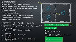
Now, shifting gears to the Hardy Cross Method. Can someone describe what we do at each node?
We assign flows and calculate head losses until they equal zero?
Spot on! It's crucial to remember that it’s not always possible to reach exactly zero. We can accept small values like less than 0.01 meters as our stopping criteria. What’s the key to finding delta Q?
It’s calculated based on the sum of head losses!
Correct! The formula for delta Q includes the sum of head losses and the cube of the head loss, aiding us in iterative adjustments. This structured approach helps confirm if our flows are properly balanced.
Introduction & Overview
Read summaries of the section's main ideas at different levels of detail.
Quick Overview
Standard
In this section, students learn about the various components of pipe networks, including different types of head losses (major and minor) that occur in a system featuring pipes with varying diameters. Detailed calculations and the Hardy Cross Method for analyzing flow in networks are introduced.
Detailed
Introduction to Pipe Networks
In pipe networks, understanding how fluid flows through pipes of various dimensions is crucial for hydraulic engineering. This section explores the concepts of head losses, which include major losses due to friction and minor losses due to changes in flow conditions, such as expansions, contractions, and valves.
Key Aspects Covered:
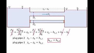
- Components of the System: The discussion begins by examining a configuration where a reservoir is connected to a pipe network that features two different diameters and a valve.
- Head Loss Calculation: Major losses are calculated using formulas tied to friction loss and the Darcy-Weisbach equation, while minor losses involve criteria such as the entrance and exit loss involving additional factors like velocity.
- Equation of Continuity: The continuity equation plays a vital role by linking flow rates and areas in different segments of the pipe system, allowing for the calculation of velocities.
- Hardy Cross Method: A mathematical approach to analyze flow in networks through iterative adjustments based on calculated flow rates and corresponding head losses is emphasized.
Overall, understanding these principles sets the foundation for deeper engagements with hydraulic systems and network design.
Youtube Videos


Audio Book
Dive deep into the subject with an immersive audiobook experience.
Understanding the Pipe Network Problem
Chapter 1 of 4
🔒 Unlock Audio Chapter
Sign up and enroll to access the full audio experience
Chapter Content
In the last class we finished the lecture by introducing a problem that is supposed to be done in the class. So there is a reservoir it is connected to a pipe, pipe is in two different areas sorry, in two different diameters. The length is the total length is 50 meter long, but this is 25 centimeter having a different diameter and this is having a different diameter. There is a sudden expansion, there is a valve here, there is going to be major losses here. And there is going to be major losses here, minor losses will be at this particular point here, here and there will also be going to be a minor loss at the square entrance.
Detailed Explanation
This chunk describes a problem involving a pipe network connected to a reservoir. The problem showcases how the reservoir is linked to a pipe of different diameters, noting that the total length of the pipe is 50 meters, and it has sections of 25 cm with varying diameters. The discussion highlights major and minor losses due to changes in the pipe's diameter and the presence of a valve, which can significantly affect the flow dynamics. Understanding these losses is crucial for analyzing fluid flow in pipe networks.
Examples & Analogies
Imagine a garden hose attached to a water source, like an outdoor faucet. If you have a section of the hose that is narrower than the rest, when you turn on the water, there will be more pressure in the faucet, but as the water reaches the narrow part of the hose, the flow speed will increase, potentially causing splashing at the exit. This is similar to how the major and minor losses work in the pipe network; when the water changes speed and diameter, it affects the overall flow.
Listing Losses in the Pipe System
Chapter 2 of 4
🔒 Unlock Audio Chapter
Sign up and enroll to access the full audio experience
Chapter Content
So we have to rewrite the total head loss H as, so starting from here it will be 0.5 V1 square/2g + 0.2 V1 square/2g + so in the pipe 1 there will be one major loss as fL v1 square/2gD1 + in pipe 2. First of all, it will be V1 – sudden expansion V1 – V2 square/ 2 g + fL2 V2 square/2gD2. This is the major loss due to the flow and in the end there is an exit loss V2 square/ 2g.
Detailed Explanation
In this chunk, the speaker outlines how to calculate the total head loss in the pipe network due to various factors including minor and major losses. They specify terms such as the head loss due to the square entrance, valve, sudden expansion, and friction within the pipes. Each type of loss is expressed with its respective formula, showcasing how they contribute to the overall loss of potential energy as water flows through the network.
Examples & Analogies
Think of riding a bike down a hill. The higher the hill, the more potential energy you have as you start. However, if there are bumps (like friction losses), or if the path suddenly narrows (like a sudden expansion), your speed and energy are affected. Just like on the bike path, when calculating water flow in pipes, you need to account for these 'bumps' which can cause losses in speed and energy.
Using the Equation of Continuity
Chapter 3 of 4
🔒 Unlock Audio Chapter
Sign up and enroll to access the full audio experience
Chapter Content
So we also know that A1 V1 = A2 V2, so A1 D1 square = A2 D2 square. So using this we can write h12 = V2 square/2g, instead of V1 sorry A1 V1 = A2 V2 sorry, so this not correct. So we can transform V1 and V2 in form of D2 and D1.
Detailed Explanation
This chunk introduces the equation of continuity, which states that the product of the cross-sectional area of a pipe (A) and the velocity of the fluid (V) at any point along the pipe remains constant for incompressible flow. This principle helps to relate the velocities in pipes of different sizes and allows for a better understanding of how changes in diameter affect flow speed. The speaker attempts to derive expressions for the head loss based on these velocities.
Examples & Analogies
Imagine a river flowing with varying widths. Where the river is narrow, the water flows faster; where it widens, the flow slows down. This concept is similar to how the equation of continuity works; it helps us understand how water speeds up or slows down as it passes through different pipe diameters.
Applying and Solving the Problem
Chapter 4 of 4
🔒 Unlock Audio Chapter
Sign up and enroll to access the full audio experience
Chapter Content
So putting this here we can get 10 = 4.03 into 4 square + 11.67 into V2 square/2g that is 76.14 into V2 square / 2g and on solution, this is going to give V2 as 1.605 meters per second and if we know V2 we can simply find Q as pi/4 into 0.30 whole square 1.605 that will give us 0.1135 meter cube per second.
Detailed Explanation
In this chunk, the speaker synthesizes the earlier equations to solve for the velocity (V2) at one end of the pipe. By substituting values into the previously established relationships, they obtain V2 as approximately 1.605 m/s and further calculate flow rate (Q) using the area of the pipe's cross-section. This process highlights the application of theoretical principles in a practical, step-by-step problem-solving context.
Examples & Analogies
Imagine turning on a faucet and noticing how quickly the water flows out. By measuring the diameter of the faucet opening and calculating the speed of the water, like the speaker does for V2, you can determine exactly how much water is flowing out every second. This is like calculating the flow rate in a pipe network, helping you understand how to regulate water usage effectively.
Key Concepts
-
Head Loss: Energy loss in a pipe system due to friction and fittings.
-
Major Loss: Friction-related losses in straight sections of pipe.
-
Minor Loss: Losses occurring at changes in flow direction or geometry.
-
Continuity Equation: Principle ensuring mass conservation in fluid flow.
-
Hardy Cross Method: Technique for analyzing flow in pipe networks through iterative calculations.
Examples & Applications
Consider a pipe system where water flows from a larger diameter pipe to a smaller one; calculate the sudden expansion loss.
In a looped piping system, applying the Hardy Cross Method to determine flow corrections for balancing.
Memory Aids
Interactive tools to help you remember key concepts
Rhymes
Friction makes flow weak, head loss we seek, both major and minor, in pipes will speak.
Stories
Once, in a pipe town, friction made the water sad, but it learned to follow routes that were less bad, impacting the flow with every turn it made.
Memory Tools
For Major and Minor losses, remember M&M, the sweet way to recall how energy dims.
Acronyms
LM = Loss of Major, and then Minor - a handy way to measure!
Flash Cards
Glossary
- Head Loss
The energy loss in a fluid system due to friction and other factors affecting flow.
- Major Loss
Head loss primarily due to friction in the pipes.
- Minor Loss
Head loss resulting from fittings such as valves, bends, and transitions.
- Continuity Equation
A fundamental principle in fluid dynamics that states that the mass flow rate must remain constant from one cross-section of a pipe to another.
- Hardy Cross Method
An iterative mathematical technique used to solve flow distribution in a network.
Reference links
Supplementary resources to enhance your learning experience.