Linear Programming
Enroll to start learning
You’ve not yet enrolled in this course. Please enroll for free to listen to audio lessons, classroom podcasts and take practice test.
Interactive Audio Lesson
Listen to a student-teacher conversation explaining the topic in a relatable way.
Introduction to Linear Programming
🔒 Unlock Audio Lesson
Sign up and enroll to listen to this audio lesson

Welcome, class! Today, we will dive into Linear Programming, often referred to as LP. It's essential because it helps us make the best decisions under constraints. Can anyone share what they think optimization means in this context?

I think optimization means making the most efficient use of resources, right?

Exactly! Optimization seeks to maximize or minimize a function, such as profits or costs. In LP, our objective is linear, involving decision variables that are essential in creating our objective function.

What kind of constraints are we talking about in LP?

Great question! Constraints are linear inequalities that limit our decision variables. We'll explore how to formulate these in the upcoming sessions. Speaking of which, can you all remember the acronym 'D.O.C.' for Decision variables, Objective function, and Constraints? Let's keep that in mind!

Got it! D.O.C. helps remember the key components.

Great teamwork! In summary, Linear Programming optimizes a linear objective function under constraints set by linear inequalities. Let's move on to how we can formulate these problems mathematically.
Mathematical Formulation
🔒 Unlock Audio Lesson
Sign up and enroll to listen to this audio lesson

Now, let's talk about how to mathematically formulate a Linear Programming Problem. It starts with defining our objective function. Can anyone recall how we express an objective function in LP?

It's in the form of Z = c₁x₁ + c₂x₂, right?

Exactly! Z is our objective to either maximize or minimize. What do the c values represent?

They are the coefficients of our decision variables.

Correct! Moving on, we list our constraints. Remember, we can express them as inequalities. Let's think about how we can visualize these constraints on a graph. What do you think our feasible region looks like?

I imagine it as a polygon formed by the intersection of the constraints.

Great visualization! In summary, the formulation of LPP involves defining decision variables, an objective function in terms of Z, and constraints as inequalities. Let's practice plotting this in our next session.
Geometric Interpretation
🔒 Unlock Audio Lesson
Sign up and enroll to listen to this audio lesson

Now that we've formulated our LPP, let’s look at how we can visualize it geometrically. Suppose we have two constraints. How do you think we can represent these on a graph?

We can plot each constraint to form a feasible region.

Correct! This feasible region shows all possible solutions that meet our constraints. Where do you think we find the optimal solution?

It’s at the vertices of the feasible region, right?

Exactly! This is known as the corner-point method. Remember, the optimum value will be at one of these vertices. Can anyone summarize the visual component of LP in one sentence?

LP problems can be visualized as feasible regions where the optimal solution lies at a vertex.

Well said! Understanding the geometric representation gives a solid grasp of where to find solutions. Next, we will discuss the various methods for solving LPPs.
Methods to Solve LPPs
🔒 Unlock Audio Lesson
Sign up and enroll to listen to this audio lesson

Let's dive into the different methods we can use to solve Linear Programming Problems. What method do you think is best for two-variable problems?

The graphical method seems ideal for that!

Absolutely! Now, what about when we have more than two variables?

We could use the Simplex Method for more complex problems.

Correct! The Simplex Method is an iterative approach that efficiently navigates vertices to find optimal solutions. There are also interior-point methods for large-scale LP problems. Can any of you summarize the key methods we discussed?

Graphical for two variables, Simplex for more, and interior-point for large problems!

Spot on! These methods are crucial to navigating LP effectively. We'll move on to the practical steps to solve these problems next.
Steps to Solve LP Problems
🔒 Unlock Audio Lesson
Sign up and enroll to listen to this audio lesson

Finally, let’s look at the steps involved in solving a Linear Programming Problem. Can anyone suggest the first step?

We need to formulate the problem with decision variables and objectives!

Exactly! Afterwards, we graph our constraints. Why is this step important?

It helps us visualize the feasible region.

Right! Following that, we plot our objective function. Can anyone explain what happens next?

We find the point where the objective function maximizes or minimizes.

Great summary! The last step is verifying our solution to ensure it meets constraints. In summary, remember the steps: formulate, graph, plot, optimize, and verify. Any questions?
Introduction & Overview
Read summaries of the section's main ideas at different levels of detail.
Quick Overview
Standard
Linear Programming (LP) is a vital optimization tool used in various fields to make decisions under resource constraints. It involves decision variables, an objective function, constraints, and non-negativity restrictions, culminating in the formulation of a Linear Programming Problem (LPP).
Detailed
Linear Programming
Introduction to Linear Programming
Linear Programming (LP) is an essential mathematical approach used for optimization, where the aim is to maximize or minimize a linear function within a set of linear constraints. The term 'linear' indicates that both the objective function and constraints are linear, involving variables only raised to the first power and multiplied by constants.
Key Components of LP
An LPP is defined by:
- Decision Variables: The unknowns we seek to solve.
- Objective Function: A linear function to be maximized or minimized.
- Constraints: A series of linear inequalities or equations that set limits on the decision variables.
- Non-negativity Restrictions: Decision variables must be greater than or equal to zero.
Mathematical Formulation
The LPP is generally formulated as:
Maximize/Minimize:  Z = c₁x₁ + c₂x₂ + ... + cₙxₙ
Subject to:
  a₁₁x₁ + a₁₂x₂ + ... + a₁ₙxₙ ≤ b₁
  a₂₁x₁ + a₂₂x₂ + ... + a₂ₙxₙ ≤ b₂
  ...
x₁, x₂, ..., xₙ ≥ 0
Here, Z is the objective function, c values are coefficients of the objective function, and a values are coefficients of constraints, while b values are constants.
Geometric Interpretation
LP problems can be represented geometrically in two dimensions with feasible regions formed by constraints. The optimum solution is found at the vertices of these regions (corner-point method).
Methods to Solve LP Problems
Several methods are available to solve LPPs:
1. Graphical Method (for two-variable problems)
2. Simplex Method (efficient for more variables)
3. Dual Simplex Method (when primal is infeasible)
4. Interior-Point Methods (for large-scale problems)
5. Software Tools (like Excel Solver) for automated solutions.
Steps to Solve LPPs
- Formulate the problem with decision variables, objective function, and constraints.
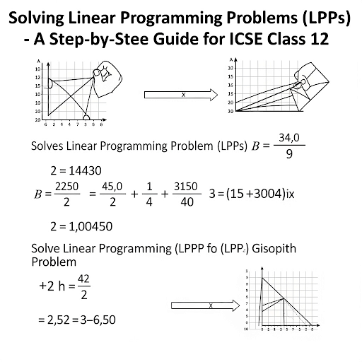
- Graph the constraints and identify the feasible region.
- Plot the objective function and optimize it.
- Verify the solution meets all constraints.
Another Example:
Types of LPPs
- Maximization Problem: Objective is to maximize profits.
- Minimization Problem: Objective is to minimize costs.
- Standard Form: Constraints in ≤ inequalities with non-negative variables.
Applications
LP is widely applicable in economics, business, and engineering, helping to resolve issues like resource allocation, transportation logistics, production planning, and more.
DOCN in Action: A Bakery Example
A bakery produces cakes and pastries. Each cake yields a profit of ₹40 and each pastry ₹30. The bakery has at most 200 hours of labor and 150 kg of flour per day.
A cake requires 4 hours and 3 kg flour; a pastry requires 2 hours and 3 kg flour. Decide how many of each to make to maximize profit.
D — Decision Variables
Let \(x\) = number of cakes, \(y\) = number of pastries.
O — Objective Function
Maximize profit:
\[
Z = 40x + 30y
\]
C — Constraints
Labor:
\[
4x + 2y \le 200
\]
Flour:
\[
3x + 3y \le 150
\]
N — Non-negativity
\[
x \ge 0,\quad y \ge 0
\]
Conclusion
Mastering fundamental LP concepts allows for effective problem-solving in optimization scenarios, aiding various decision-making processes under constraints.
Linear Programming (LP) — Worked Example
A. Diet Problem — Full LP Formulation + Graphical Solution
1) Problem Statement
Choose quantities of two foods to meet nutrition needs at minimum cost.
| Food | Cost (₹/serving) | Calories | Protein (g) |
|---|---|---|---|
| A | 30 | 400 | 10 |
| B | 20 | 200 | 6 |
Daily requirements: at least 1200 calories and 36 g protein.
2) Decision Variables
Let
- \(x \ge 0\) = servings of Food A
- \(y \ge 0\) = servings of Food B
3) Objective (Minimize Cost)
\[
\min \ C = 30x + 20y
\]
4) Constraints (Nutrition)
- Calories: \(400x + 200y \ge 1200 \ \Rightarrow\ 2x + y \ge 6\)
- Protein: \(10x + 6y \ge 36 \ \Rightarrow\ 5x + 3y \ge 18\)
- Non-negativity: \(x \ge 0,\ y \ge 0\)
5) Graphical Method (Two-Variable LP)
Plot the lines:
- \(2x + y = 6\) (region above the line is feasible)
- \(5x + 3y = 18\) (region above the line is feasible)
Corner points of the feasible region (check intersections with axes and each other):
- Intersection with axes for \(2x + y = 6\):
- \(x=0 \Rightarrow y=6\) → \((0,6)\)
- \(y=0 \Rightarrow x=3\) → \((3,0)\) (but check protein)
- Intersection with axes for \(5x + 3y = 18\):
- \(x=0 \Rightarrow y=6\) → \((0,6)\)
- \(y=0 \Rightarrow x=\tfrac{18}{5}=3.6\) → \((3.6,0)\)
-
Intersection of the two lines:
Solving
\[
\begin{cases}
2x + y = 6 \
5x + 3y = 18
\end{cases}
\Rightarrow x=0,\ y=6 \ (\text{same as } (0,6)).
\]
Feasibility check & cost at corner points:
- \((3,0)\): Protein \(=5(3)+3(0)=15 < 18\) ⇒ infeasible.
- \((0,6)\): Feasible. Cost \(C = 30(0)+20(6)=120\).
- \((3.6,0)\): Feasible. Cost \(C = 30(3.6)+20(0)=108\).
Optimal Solution (Minimum Cost):
Alright 👍 here it is in a plain copyable format (not markdown):
x⁎ = 3.6, y⁎ = 0, Cₘᵢₙ = ₹108
Interpretation: Choose 3.6 servings of Food A and 0 of B to meet both requirements at the lowest cost.
Tip: In diet problems, fractional servings are allowed (continuous decision variables).
B. (Optional) LP Tableau Illustration (Maximization Example)
To see an LP tableau, it’s simpler to use a standard maximization with “\(\le\)” constraints (no artificial variables needed initially).
Example
Maximize \(Z = 5x + 4y\)
Subject to
\[
\begin{aligned}
6x + 4y &\le 24 \
x + 2y &\le 6 \
x, y &\ge 0
\end{aligned}
\]
Add slack variables \(s_1, s_2 \ge 0\):
\[
\begin{aligned}
6x + 4y + s_1 &= 24 \
x + 2y + s_2 &= 6
\end{aligned}
\]
Initial Simplex Tableau
| Basic Var | x | y | s₁ | s₂ | RHS |
|---|---|---|---|---|---|
| s₁ | 6 | 4 | 1 | 0 | 24 |
| s₂ | 1 | 2 | 0 | 1 | 6 |
| Z-row | -5 | -4 | 0 | 0 | 0 |
- Entering variable: \(x\) (most negative in Z-row: \(-5\))
- Leaving variable: ratio test → \(24/6 = 4\) vs \(6/1 = 6\) ⇒ row 1 leaves (pivot at 6).
(You can continue the usual Simplex steps—normalize pivot row, eliminate \(x\) from others—to reach the optimal solution. Graphically, this one reaches optimum at \((x,y)=(2,2)\) with \(Z=18\).)
Youtube Videos


Audio Book
Dive deep into the subject with an immersive audiobook experience.
Introduction to Linear Programming
Chapter 1 of 1
🔒 Unlock Audio Chapter
Sign up and enroll to access the full audio experience
Chapter Content
Linear Programming (LP) is a mathematical technique used for optimization, where the objective is to maximize or minimize a linear function subject to a set of linear constraints. The term "linear" refers to the fact that both the objective function and the constraints are linear (i.e., they involve only variables raised to the power of 1 and multiplied by constants).
Detailed Explanation
Linear Programming (LP) is a method used to find the best possible outcome in a given situation. It focuses on maximizing or minimizing a certain value—this is called the objective function. This function is 'linear,' meaning it can be represented with straight lines on a graph. Additionally, there are constraints, which are limitations or requirements we must follow while making our decisions. LP is commonly used in various fields like economics, business, and engineering where resource management is essential.
Examples & Analogies
Imagine you run a small bakery. You have limited resources, such as flour, sugar, and eggs. Your goal is to maximize the number of cakes you can sell. If you know how much of each ingredient is available (your constraints) and how much profit each type of cake makes (your objective function), you can use linear programming to determine the best mix of cakes to bake. This way, you can make the most money with your limited resources.
Key Concepts
-
Linear Programming (LP): A method to achieve the best outcome under constraints.
-
Decision Variables: Unknowns we solve in LP.
-
Objective Function: Function to maximize or minimize.
-
Constraints: Limitations in LP, defined by linear inequalities.
-
Feasible Region: Area satisfying all constraints.
-
Simplex Method: An efficient algorithm for determining optimal solutions.
Examples & Applications
In maximizing profit for a factory, LP can determine the optimal number of products to manufacture given raw material and labor constraints.
Using LP in transportation problems could minimize shipping costs while adhering to supply and demand constraints.
Memory Aids
Interactive tools to help you remember key concepts
Rhymes
When you want to optimize, remember LP will advise, with variables, constraints and functions wise.
Stories
Imagine a farmer deciding on which crops to plant for maximum yield. By applying LP, they find the ideal balance under their resource constraints.
Memory Tools
Remember 'D.O.C.' for Decision variables, Objective function, and Constraints!
Acronyms
For steps to solve, remember F-G-P-O-V
Formulate
Graph
Plot
Optimize
Verify.
Flash Cards
Glossary
- Decision Variables
Unknown variables in an LP problem that we need to solve for.
- Objective Function
The function that needs to be maximized or minimized in an LP problem.
- Constraints
Linear inequalities or equations that restrict the values of decision variables.
- Feasible Region
The set of all possible points that satisfy the constraints in an LP problem.
- Simplex Method
An efficient algorithm for solving LP problems with more than two variables.
- Graphical Method
A visual approach to solving LP problems involving two variables.
- Nonnegativity Restrictions
Conditions stating that decision variables must be greater than or equal to zero.
- Cornerpoint Method
A technique used in LP to find optimal solutions at the vertices of the feasible region.
