
Block Diagram Representation of CT-LTI Systems: A Visual Language
Interactive Audio Lesson
Listen to a student-teacher conversation explaining the topic in a relatable way.
Building Blocks of CT-LTI Systems
🔒 Unlock Audio Lesson
Sign up and enroll to listen to this audio lesson

Today, we’re going to discuss the various building blocks of continuous-time linear time-invariant systems represented in block diagrams. Can anyone tell me what an adder or summing junction does?

Is it where you combine different signals?
Correct! An adder, represented by a circle with a cross, sums multiple input signals into one output signal. Next, who can describe the scalar multiplier?

It's a block that multiplies an input by a constant, right?
Exactly! Now let's look at the integrator and differentiator; why do you think we prefer integrators over differentiators?

Because differentiators can amplify noise?
Yes! Integrators help avoid this issue. Remember, integration is typically more stable. Let’s summarize. We discussed the adder, gain block, integrator, and differentiator, focusing especially on their purposes in signal processing.
Direct Form I and Direct Form II Realization
🔒 Unlock Audio Lesson
Sign up and enroll to listen to this audio lesson

Now that we know the basic blocks, let’s discuss how to implement these in practice. What do we mean by Direct Form I realization?

It's where the differential equation structure is split for input and output operations?
Exactly! In Direct Form I, we separate the input and output derivatives, leading to a more straightforward translation of the LCCDE. Student_2, can you explain how Direct Form II differs?
Direct Form II uses fewer integrators and is optimized for efficiency, right?
Great! It streamlines the operations, using only 'N' integrators for an N-th order system. Why might this be beneficial in signal processing?
It reduces memory requirements and improves performance!
Correct! Let’s recap. We explored Direct Form I and Direct Form II, noting their construction methods and advantages.
Interconnections of CT-LTI Systems
🔒 Unlock Audio Lesson
Sign up and enroll to listen to this audio lesson
Lastly, let’s look at how systems can be interconnected. What do we mean by cascade interconnection?
It's where the output of one system becomes the input of another!
Exactly! This allows us to create complex systems easily. What about parallel interconnection, Student_4?
That’s when multiple systems receive the same input signal and their outputs are summed up.
Nice! And what about feedback interconnections?
That’s when a part of the output goes back to the input, usually to stabilize the system.
Absolutely right! Feedback is crucial for maintaining control in systems. To sum up, we’ve discussed cascade, parallel, and feedback interconnections in block diagrams.
Introduction & Overview
Read summaries of the section's main ideas at different levels of detail.
Quick Overview
Standard
Block diagrams are essential tools for visualizing continuous-time systems. This section discusses various blocks, such as summing junctions, multipliers, integrators, and differentiators, as well as two realization forms—Direct Form I and Direct Form II—demonstrating how to implement differential equations in practical applications.
Detailed
Block Diagram Representation of CT-LTI Systems
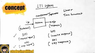
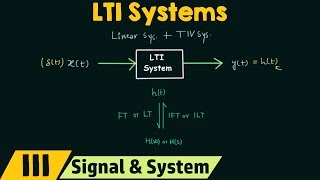
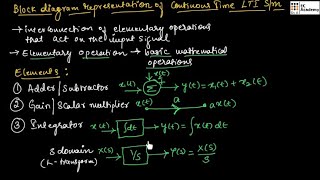
Block diagrams serve as a vital visual language for analyzing and designing continuous-time linear time-invariant (CT-LTI) systems. This section presents the fundamental building blocks that make up a block diagram, including adders, multipliers, integrators, and differentiators. Each block has a unique function, contributing to the overall system.
Building Blocks
- Adder/Summing Junction: This block allows multiple input signals to be summed into a single output, indicated through a circle with a cross inside. The sum can either be algebraic addition or subtraction.
- Scalar Multiplier/Gain Block: Represented by a rectangle containing a constant, this block scales an input signal by a defined constant value.
- Integrator: Crucial for implementing differential equations, this block produces the integral of its input with respect to time.' It is symbolized by a rectangle with an integral sign and is utilized instead of differentiation to minimize noise sensitivity.
- Differentiator: Though not commonly used in practical implementations due to noise amplification, this block mathematically obtains the derivative of an input signal.
- Connection Lines: Arrows between blocks indicate the flow of signals, directing how signals move through the system.
Realization Forms
Two primary methods to realize block diagrams are:
- Direct Form I: This realization breaks down a differential equation structure into two sections: one for input operations and another for output. It requires multiple integrators and produces a diagram that closely mirrors the differential equation's format.
- Direct Form II: Optimized for efficiency, this form reduces the number of integrators needed, utilizing only 'N' integrators for an N-th order system. It reorganizes operations for better performance.
Interconnections
Block diagrams are invaluable for showing how different LTI systems combine to form complex systems. These combinations can be in series (cascaded), parallel (simultaneous), or feedback configurations, each with important implications for system design and analysis.
Youtube Videos


Audio Book
Dive deep into the subject with an immersive audiobook experience.
Building Blocks of CT-LTI Systems
Chapter 1 of 4
🔒 Unlock Audio Chapter
Sign up and enroll to access the full audio experience
Chapter Content
Building Blocks of CT-LTI Systems:
- Adder/Summing Junction: Represented by a circle with a cross inside. Multiple input signals enter, and a single output signal is their algebraic sum. Signs (+/-) indicate addition or subtraction.
- Scalar Multiplier/Gain Block: Represented by a rectangle with a constant 'K' inside. An input signal is multiplied by the constant 'K' to produce the output.
- Integrator: Represented by a rectangle with an integral sign (or 1/s in the Laplace domain context, though we are in time domain here). Its output is the integral of its input with respect to time. This is a crucial element for realizing differential equations because differentiation is often avoided due to noise sensitivity. Integration is the stable, preferred operation.
- If input is f(t), output is integral of f(tau) d(tau) (from some initial time to t).
- Differentiator: Represented by a rectangle with d/dt (or 's' in the Laplace domain). Its output is the derivative of its input. While mathematically valid, practical implementations often avoid differentiators because they amplify high-frequency noise.
- Connection Lines (Arrows): Indicate the direction of signal flow between blocks.
Detailed Explanation
Block diagrams consist of basic components that represent different operations in continuous-time linear time-invariant (CT-LTI) systems. The 'Adder/Summing Junction' allows multiple input signals to come together into a single output that is the sum of the inputs, whether they are added or subtracted. The 'Scalar Multiplier' serves the purpose of scaling an input signal by a constant factor, which alters the output accordingly. When you need to integrate a signal over time—such as in solving differential equations—the 'Integrator' block is essential, providing a stable option over differentiators that may be sensitive to noise. The 'Differentiator' block, in contrast, produces the rate at which a signal changes but is less desirable in practice due to its susceptibility to noise. Finally, arrows or lines in these diagrams denote the flow of signals between these operations, giving a clear visual representation of how the signals interact within the system.
Examples & Analogies
Imagine a music mixing board in a recording studio: the 'Adder/Summing Junction' acts like the mixer that takes different sound inputs (vocals, instruments) and combines them into a single audio output. The 'Scalar Multiplier' can be likened to the volume knob that increases or decreases the intensity of a sound. The 'Integrator' can be thought of as a digital effect that creates reverb, adding depth to a sound, whereas the 'Differentiator' might resemble a feature that sharpens or alters the dynamics of sound inputs but can introduce unwanted noise. Together, these components help create a harmonious final sound, represented visually in the block diagram.
Direct Form I Realization: A Straightforward Translation
Chapter 2 of 4
🔒 Unlock Audio Chapter
Sign up and enroll to access the full audio experience
Chapter Content
Direct Form I Realization: A Straightforward Translation
- Concept: This realization directly implements the differential equation structure by separating the operations on the input and output derivatives. It involves two main parts: one for the input derivatives and one for the output derivatives, connected in series.
- Procedure for Construction (for an N-th order LCCDE):
- Rearrange the LCCDE to express the highest derivative of the output in terms of all other terms. For example, for a second-order system:
d^2 y(t)/dt^2 = (1/a_2) * [b_2 * d^2 x(t)/dt^2 + b_1 * dx(t)/dt + b_0 * x(t) - a_1 * dy(t)/dt - a_0 * y(t)] - Identify a conceptual intermediate signal, often denoted w(t), such that integrating w(t) N times yields y(t). This is sometimes referred to as the output of the integration chain before scaling.
- Create a chain of N integrators, where the output of the last integrator is y(t), the output of the second-to-last is y'(t), and so on, up to y^(N-1)(t).
- Create a similar chain for the input derivatives, but typically the input derivatives are summed first.
- Realize the right-hand side of the rearranged equation: Implement the derivatives of the input signal using differentiators (though integrators are preferred for practical realizations as discussed below).
- Sum the scaled input and its derivatives.
- Sum the scaled output and its derivatives (with negative signs if moved to the right side of the equation).
- The sum of these scaled and differentiated signals then feeds the first integrator in the output chain.
- The result will be a block diagram with separate "input-side" and "output-side" sections.
Detailed Explanation
The Direct Form I realization provides a schematic way to translate the structure of a differential equation into a block diagram. It takes the differential equation used to describe the system's dynamics and rearranges it to focus on the highest order of the output's derivative. After this rearrangement, an intermediate signal is identified to facilitate the process of integrating back to the output signal. This method involves connecting several integrators in a sequence based on the order of the differential equation, which allows for a straightforward implementation of how input and output signals are related. Essentially, this realizes how the response changes based on the state of past outputs and input values, hence producing clear visual and practical representations of on-going continuous processes in the CT-LTI system.
Examples & Analogies
Think of a Direct Form I realization like adjusting the settings on a home heating system. You start by defining the main control (the thermostat) that reacts to the temperature of the house (the output). To get the actual temperature reading, you may set several levels—like the current temperature, desired temperature, and other conditions that you need to keep track of. Each setting adjustment or change corresponds to an integrator in the block diagram. The way the heating responds by adding heat based on these settings is analogous to how the integrators sum up the effects of past inputs and outputs to achieve a stable final temperature.
Direct Form II Realization: Optimized for Efficiency
Chapter 3 of 4
🔒 Unlock Audio Chapter
Sign up and enroll to access the full audio experience
Chapter Content
Direct Form II Realization: Optimized for Efficiency
- Concept: This realization is derived from Direct Form I by exploiting the linearity and associativity of LTI systems. It often uses fewer integrators, specifically only 'N' integrators for an N-th order system, regardless of 'M'. It reorders the operations such that all integrations are performed first on an intermediate signal, and then scaling and summation operations are performed.
- Procedure for Construction:
- Start with the general LCCDE form.
- Introduce a conceptual intermediate signal, w(t), such that:
- The input x(t) is fed into a "system" that generates w(t) based on the input derivative terms (b_k coefficients). This section involves differentiators or an integrator chain.
- The output y(t) is then generated from w(t) based on the output derivative terms (a_k coefficients). This section effectively "filters" w(t) using the output's characteristic equation.
- More commonly, we view it as:
- Feed x(t) into a series of 'N' integrators. The output of the last integrator is an intermediate signal, say v(t).
- Take signals from the input to each integrator (x(t), integral of x(t), etc.) and scale them by the b_k coefficients, then sum them to form w(t).
- Take signals from the output of each integrator (v(t), integral of v(t), etc.) and scale them by the a_k coefficients, then sum them and subtract them from w(t) to form the input to the first integrator.
- This is typically achieved by rearranging the equation and implementing the input side's transfer function first, followed by the output side's inverse transfer function.
- A key simplification arises from implementing the "zeros" (M part) and "poles" (N part) of the system function with shared integrators.
Detailed Explanation
Direct Form II realization enhances the efficiency of representing differential equations through block diagrams. This method reduces the number of integrators needed by focusing on the structural properties of LTI systems. Essentially, instead of separately addressing the input and output in a cumbersome way, it rearranges inputs to derive an intermediate signal and process all integrations in a streamlined fashion. Thus, this leads to a simplified implementation in which the same integrators can be used for both the generation of system responses and the application of system characteristics. It results in a more compact and efficient layout, conserving resources without sacrificing clarity or function.
Examples & Analogies
Consider a chef preparing a meal that can be efficiently done in a single pot instead of multiple pans and dishes. In this sense, Direct Form II realization embodies this cooking method where all ingredients (inputs) are added and stirred together (integrated) first to create a base sauce (intermediate signal), which is then seasoned and adjusted (output processing) for the final dish (output). Just like the chef’s streamlined approach saves time and effort, this realization in signal processing optimizes the use of computational resources while maintaining a clean and functional setup.
Interconnections of CT-LTI Systems: Building Complex Systems from Simple Blocks
Chapter 4 of 4
🔒 Unlock Audio Chapter
Sign up and enroll to access the full audio experience
Chapter Content
Interconnections of CT-LTI Systems: Building Complex Systems from Simple Blocks
- Block diagrams are particularly useful for representing how individual LTI systems are combined to form more complex systems.
- Cascade Interconnection (Series Connection):
- Description: The output of one system serves as the input to the next system. If system 1 has impulse response h1(t) and system 2 has impulse response h2(t), and they are cascaded, then y(t) = [x(t) * h1(t)] * h2(t).
- Overall Impulse Response: Due to the associative property of convolution, the overall equivalent impulse response of cascaded LTI systems is the convolution of their individual impulse responses: h_eq(t) = h1(t) * h2(t).
- Diagram: A series of rectangles connected by arrows, where the output of one feeds into the input of the next.
- Significance: Allows for modular design and analysis. The order of LTI systems in cascade can be interchanged without affecting the overall input-output relationship.
- Parallel Interconnection:
- Description: The same input signal is applied simultaneously to multiple systems, and their individual outputs are summed to produce the overall output. If system 1 has h1(t) and system 2 has h2(t), then y(t) = (x(t) * h1(t)) + (x(t) * h2(t)).
- Overall Impulse Response: Due to the distributive property of convolution, the overall equivalent impulse response of parallel LTI systems is the sum of their individual impulse responses: h_eq(t) = h1(t) + h2(t).
- Diagram: A single input line splitting to feed multiple parallel rectangles, with their outputs converging into an adder.
- Significance: Used to combine the effects of different system components or to create filters with specific response characteristics.
- Feedback Interconnection:
- Description: The output, or a portion of the output, is fed back to the input, often with a gain or through another system, and typically subtracted from the original input. This creates a closed-loop system.
- Diagram: A loop where the output signal (or a derived signal from the output) is routed back to an adder at the input.
- Significance: Crucial for control systems, for stabilizing unstable systems, shaping system responses, and for oscillators. Analyzing feedback systems typically requires techniques from the Laplace domain (covered in later modules), as direct time-domain analysis becomes very complex.
Detailed Explanation
Block diagrams can illustrate the intricate relationships between various LTI systems, showing how they can be interconnected to construct complex system dynamics. Cascade interconnections link systems in series, allowing the output of one to be directly influenced by the input of the next. This relationship forms the basis for understanding overall system behavior as represented through the convolution of impulse responses from each system. On the other hand, parallel connections showcase how multiple systems can simultaneously process the same input and contribute to a combined output, demonstrating flexibility in how systems might operate together. Finally, feedback interconnections feed elements of output back into the system to refine or adjust the input, vital for control mechanisms and stability considerations within the systems.
Examples & Analogies
Think of building a themed amusement park, where rides represent different LTI systems. In a cascade interconnection, a train ride (System 1) smoothly leads into a funhouse (System 2)—the output of the train ride becomes the input for the funhouse, creating a continuous flow of excitement. In parallel interconnection, you could have a group of cafes, all serving refreshments to hungry patrons simultaneously—each café processes the same influx of guests, adding to the overall atmosphere. For feedback interconnection, imagine a roller coaster where riders can choose how fast to go by pulling on a brake lever—this mechanism adjusts the ride dynamically based on the output (speed) and directly influences the experiences of the next riders.
Key Concepts
-
Adder/Summing Junction: Combines multiple input signals into one output.
-
Scalar Multiplier: Scales an input signal by a constant.
-
Integrator: Generates the integral of an input signal.
-
Differentiator: Produces the derivative of an input signal.
-
Direct Form I: Direct representation of a differential equation.
-
Direct Form II: Optimized representation using fewer components.
-
Cascade Interconnection: Chains systems together.
-
Parallel Interconnection: Applies one signal simultaneously to multiple systems.
-
Feedback Interconnection: Routes output back to the input for control.
Examples & Applications
The use of a square wave signal combined with multiple filters in a sound system can be analyzed using a block diagram.
A feedback control loop in an automated thermostat can be represented using block diagrams.
Memory Aids
Interactive tools to help you remember key concepts
Rhymes
An adder adds with such delight, two signals combined just feels right.
Stories
Once in a signal town, an adder met a multiplier. Together they combined and scaled, creating a harmonious output for the whole community.
Memory Tools
Remember 'AIM' for block diagrams: A is for Adder, I for Integrator, M for Multiplier.
Acronyms
For the realization forms, think 'DFI' for Direct Form I and 'DFII' for Direct Form II.
Flash Cards
Glossary
- Adder/Summing Junction
A block that sums multiple input signals into a single output signal.
- Scalar Multiplier/Gain Block
A block that scales an input signal by a constant.
- Integrator
A block that outputs the integral of its input signal over time.
- Differentiator
A block that outputs the derivative of its input signal.
- Direct Form I Realization
A method of implementing a system based on the differential equation structure, separating input and output operations.
- Direct Form II Realization
An optimized method of implementing a system that minimizes the number of integrators used.
- Cascade Interconnection
A configuration where the output of one system is the input to another.
- Parallel Interconnection
A configuration where multiple systems receive the same input and their outputs are summed.
- Feedback Interconnection
A configuration that routes a portion of the output back to the input.
Reference links
Supplementary resources to enhance your learning experience.