
Traffic Stream Models
Enroll to start learning
You’ve not yet enrolled in this course. Please enroll for free to listen to audio lessons, classroom podcasts and take practice test.
Interactive Audio Lesson
Listen to a student-teacher conversation explaining the topic in a relatable way.
Introduction to Traffic Stream Models
🔒 Unlock Audio Lesson
Sign up and enroll to listen to this audio lesson

Good morning class! Today we're diving into traffic stream models, which are essential for analyzing traffic behavior. Who can tell me why understanding traffic parameters like speed and density is important?

It helps manage traffic flow and reduce congestion!
Exactly! We need reliable models to predict traffic conditions. Let's start with Greenshield's model. Can anyone explain what it relates?

It's about the relationship between speed and density!
That's right! Remember, as density increases, speed can decrease. To help you remember, think of the acronym 'SLOPE' (Speed, Loss, Over density, Predicts flow, Effects traffic).

So if speed decreases, does that mean density goes up?
Exactly! As more vehicles enter a given space, speed tends to decrease. Let's summarize this: understanding speed-density relationships helps us predict flow patterns.
Calculating Maximum Flow
🔒 Unlock Audio Lesson
Sign up and enroll to listen to this audio lesson

Next, let’s calculate the maximum flow using Greenshield's model. Who remembers the equation?

Isn’t it related to jam density and free flow speed?
Good recall! The maximum flow can be determined to be one-fourth of the product of these two variables. What do you think this tells us about traffic capacity?
It shows that there’s an optimal point where flow is maximized!
Exactly! Let's say we have a free flow speed of 70 km/hr and a jam density of 200 veh/km, can anyone calculate the maximum flow?
It would be 70 times 200 divided by 4, which equals 3500 veh/hr!
Perfect! So always remember to check your calculations when dealing with traffic stream models.
Calibration of Models
🔒 Unlock Audio Lesson
Sign up and enroll to listen to this audio lesson
Now, let’s turn to the application of Greenshield's model. What does calibration mean in this context?
Is it about adjusting the model based on actual data?
Yes! Calibration helps us align model predictions with real-world measurements. Can anyone give examples of parameters we might calibrate?
Free flow speed and jam density!
Exactly! We derive these from field data and perform regression analysis. Can anyone share how we might approach this calculation?
By performing linear regression on the data points we observed!
Correct! Always remember: real data informs model accuracy. Let's summarize: calibrating ensures our models reflect reality.
Understanding Alternative Models
🔒 Unlock Audio Lesson
Sign up and enroll to listen to this audio lesson
We've seen Greenshield's linearity, but what about other models?
There’s Greenberg's logarithmic model!
Great mention! Greenberg’s model uses logarithmic relationships. What do you think is a limitation of that?
It tends toward infinite speeds at low densities!
Exactly! Other models like Underwood's and Pipe’s offer different perspectives as well. Why do you think we need multiple models?
To account for varying traffic conditions!
Precisely! Different scenarios call for tailored approaches. Always keep this diversity in models in mind.
Introduction & Overview
Read summaries of the section's main ideas at different levels of detail.
Quick Overview
Standard
This section provides an overview of traffic stream models, particularly highlighting Greenshield’s macroscopic model, which illustrates the relationship between traffic parameters such as speed, density, and flow. It also compares Greenshield’s model with other models and presents methodologies to calibrate and apply these models in practical scenarios.
Detailed
Traffic Stream Models - Detailed Summary
Traffic stream models are mathematical representations used to elucidate relationships among various traffic parameters such as speed, density, and flow. Over decades, extensive research has contributed to the development of these models, enabling better analysis and management of traffic conditions.
Key Models Discussed:
1. Greenshield’s Macroscopic Stream Model
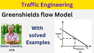
Greenshield's model is crucial in understanding the linear relationship between speed (v) and density (k). The fundamental equation is given by:
Where:
- v = Mean speed at density k
- v_f = Free-flow speed, and
- k_j = Jam density.
This implies that as density approaches zero, speed approaches free-flow conditions. Subsequent derivations relate flow and density, revealing a parabolic relationship unresolved in the Greenshield model.
The maximum flow (q_max) can be calculated via differentiation and is found to equal one-fourth of the product of free-flow speed and jam density.
2. Calibration of Greenshield’s Model
Calibration is essential for practical application. Free flow speeds and jam densities are determined from field surveys, and linear regressions are performed to fit observed data. Equations derived for coefficients a and b help describe traffic settings accurately.
3. Other Models
In response to limitations in Greenshield's linearity, other models emerged:
- Greenberg’s Logarithmic Model: Captures logarithmic speeds with density, but fails at low densities.
- Underwood’s Exponential Model: Represents exponential relationships but struggles with high-density predictions.
- Pipe’s Generalized Model: Adds flexibility with a parameter for varied density conditions.
- Multiregime Models: Account for behavioral changes across different density ranges.
4. Shock Waves
Shock waves in traffic reflect abrupt changes, like accidents or obstructions, indicating a cascading effect in vehicle flow. The propagation of density-state changes can be analyzed with equations derived for speed and flow in these scenarios.
Overall, understanding these models is fundamental for transportation engineering principles aimed at managing and forecasting traffic flow effectively.
Youtube Videos


Audio Book
Dive deep into the subject with an immersive audiobook experience.
Overview of Traffic Stream Models
Chapter 1 of 9
🔒 Unlock Audio Chapter
Sign up and enroll to access the full audio experience
Chapter Content
To figure out the exact relationship between the traffic parameters, a great deal of research has been done over the past several decades. The results of these researches yielded many mathematical models. Some important models among them will be discussed in this chapter.
Detailed Explanation
This chunk introduces the general purpose of traffic stream models, which is to understand the relationships between various traffic parameters. Traffic parameters can include speed, density, and flow of vehicles on a roadway. Research conducted over several decades has led to the development of mathematical models that describe these relationships, and the chapter will focus on some key models that are particularly significant.
Examples & Analogies
Think of traffic stream models like a recipe for cooking. Just as a recipe lists ingredients and their quantities to create a dish, traffic models list different traffic parameters and how they interact to describe traffic conditions. By following the recipe (or model), traffic engineers can predict how vehicles will behave in various situations.
Greenshield's Macroscopic Stream Model
Chapter 2 of 9
🔒 Unlock Audio Chapter
Sign up and enroll to access the full audio experience
Chapter Content
Macroscopic stream models represent how the behaviour of one parameter of traffic flow changes with respect to another. Most important among them is the relation between speed and density. The first and most simple relation between them is proposed by Greenshield.
Detailed Explanation
Macroscopic stream models look at aggregate traffic behavior, focusing on how one traffic parameter affects another. Greenshield proposed a straightforward linear relationship between the speed of vehicles and the density of vehicles on the road. In this model, as the density increases, speed decreases. This relationship helps to understand how vehicle flow behaves under different traffic conditions and is foundational in traffic engineering.
Examples & Analogies
Imagine a highway during rush hour. As more cars enter the road (increasing density), each car has less space to move. Consequently, they slow down, which illustrates the Greenshield’s model. It's similar to people in a crowded elevator—when there are too many people, it becomes hard to move freely.
Greenshield's Equation
Chapter 3 of 9
🔒 Unlock Audio Chapter
Sign up and enroll to access the full audio experience
Chapter Content
The equation for this relationship is shown below:
v_f
v = v_f . k / (k_j - k) (33.1)
Detailed Explanation
In this equation, 'v' represents the mean speed at a given density 'k', 'v_f' is the free flow speed (the speed limit in ideal conditions), and 'k_j' refers to jam density (the point where traffic is stopped completely). The equation shows how speed reduces as the density increases until it reaches jam density. At zero density, the speed approaches 'v_f'.
Examples & Analogies
Consider a water hose. When water flows freely (no blockage), it moves quickly. But if you pinch the hose (like increasing density), the flow slows down. The Greenshield's equation captures this concept mathematically by establishing how speed changes with density.
Flow-Density Relationship
Chapter 4 of 9
🔒 Unlock Audio Chapter
Sign up and enroll to access the full audio experience
Chapter Content
Once the relation between speed and flow is established, the relation with flow can be derived. This relation between flow and density is parabolic in shape.
Detailed Explanation
After understanding the relationship between speed and density, the next step is to analyze flow with respect to density. This relationship takes on a parabolic shape, showing how flow increases with density up to a certain point before it starts to decrease again. The peak of the parabola represents the maximum flow capacity of the road.
Examples & Analogies
Imagine a concert where everyone rushes to enter. Initially, the crowd builds up (density increases) and more people can get in the venue (flow increases), but if it gets too crowded, it becomes hard to move, and fewer people can enter (flow decreases). The relationship between flow and density in traffic is quite similar.
Maximum Flow and Density
Chapter 5 of 9
🔒 Unlock Audio Chapter
Sign up and enroll to access the full audio experience
Chapter Content
The boundary conditions that are of interest are jam density, free-flow speed, and maximum flow. To find density at maximum flow, differentially equation 33.3 with respect to k and equate it to zero.
Detailed Explanation
To determine maximum flow, traffic engineers look for specific boundary conditions, such as jam density and free-flow speed. By applying calculus to the flow-density equation, they can find the density at which maximum flow occurs. This is significant for road design and traffic management.
Examples & Analogies
Think of a water tank. There’s a point where you can fill it (maximum flow) effectively before it overflows (jam density). By measuring how full the tank gets before it starts spilling over, you can determine the best way to manage water levels—just like finding optimal traffic flow conditions.
Calibration of Greenshield's Model
Chapter 6 of 9
🔒 Unlock Audio Chapter
Sign up and enroll to access the full audio experience
Chapter Content
In order to use this model for any traffic stream, one should get the boundary values, especially free flow speed (v_f) and jam density (k_j). This has to be obtained by field survey and this is called calibration process.
Detailed Explanation
Calibration involves gathering real-world data to establish the specific parameters needed for Greenshield's model—namely free-flow speed and jam density. This process involves conducting field surveys and analyzing observed traffic data to identify these key values, making the model applicable in practical scenarios.
Examples & Analogies
Calibrating the model can be likened to tuning a musical instrument. Just as a musician needs to adjust strings based on what they hear to ensure proper sound, traffic engineers must collect data and adjust model parameters so they accurately reflect real traffic conditions.
Limitations of Greenshield's Model
Chapter 7 of 9
🔒 Unlock Audio Chapter
Sign up and enroll to access the full audio experience
Chapter Content
In Greenshield’s model, linear relationship between speed and density was assumed. But in field, we can hardly find such a relationship between speed and density. Therefore, the validity of Greenshields’ model was questioned and many other models came up.
Detailed Explanation
While Greenshield's model provides a foundation for understanding traffic flow, it operates on the linearity assumption, which may not accurately depict real-world complexities under varied traffic conditions. As such, traffic researchers have proposed alternative models that better capture the relationships observed on actual roadways, showing that these relationships can be non-linear.
Examples & Analogies
Consider weather predictions. Early models were based on simple linear assumptions about temperature changes, but actual weather patterns are quite complex and often require more intricate models that account for variations. Similarly, traffic models must adapt to complexities to remain valid.
Other Macroscopic Stream Models
Chapter 8 of 9
🔒 Unlock Audio Chapter
Sign up and enroll to access the full audio experience
Chapter Content
Prominent among them are Greenberg’s logarithmic model, Underwood’s exponential model, Pipe’s generalized model, and multiregime models.
Detailed Explanation
This chunk introduces alternative models developed to address the limitations of the Greenshield model. Concepts such as logarithmic, exponential, and generalized models offer different ways of understanding the speed-density relationship, each with its advantages and shortcomings in their applications to traffic flow.
Examples & Analogies
You can think of these models like different styles of cooking. Just as a chef might choose a baking, frying, or steaming method based on the dish they wish to prepare, traffic engineers select different models based on the traffic conditions they’re assessing.
Shock Waves in Traffic
Chapter 9 of 9
🔒 Unlock Audio Chapter
Sign up and enroll to access the full audio experience
Chapter Content
The flow of traffic along a stream can be considered similar to a fluid flow. The sudden change in the characteristics of the stream leads to the formation of a shock wave.
Detailed Explanation
Shock waves occur in traffic systems when sudden changes—like an accident or road block—impact the uniform flow of vehicles. This sudden disruption can cause vehicles further back to slow down, creating a wave effect that travels upstream. Understanding shock waves can be critical for traffic management and mitigation strategies.
Examples & Analogies
Think of a line of dominoes. When one domino falls, it causes a chain reaction affecting others. Similarly, in traffic, when an event occurs, it can set off a chain reaction of slowing down or stopping vehicles, creating shock waves in the traffic flow.
Key Concepts
-
Traffic Parameters: Concepts like speed, density, and flow that are fundamental to traffic flow analysis.
-
Greenshield's Model: A foundational model that uses a linear relationship between speed and density.
-
Calibration: Adjusting model parameters based on empirical data to ensure accuracy in predictions.
-
Maximum Flow: The peak rate of vehicle flow that can occur under optimal traffic conditions.
Examples & Applications
If the jam density is 200 vehicles/km and the free flow speed is 70 km/hr, the maximum flow would be calculated as 3500 vehicles/hr.
Using field data, traffic engineers can determine the free flow speed and jam density needed to calibrate Greenshield's model.
Memory Aids
Interactive tools to help you remember key concepts
Rhymes
Speed is fast, density is tight, together they show traffic's plight.
Stories
Imagine a river where water flows smoothly when it's wide apart, but jams occur when things get tight, just like traffic in a busy part.
Memory Tools
For Greenshield’s maximum flow, remember '1/4 Free Speed times Jam Density' to guide your calculations.
Acronyms
Use 'FLUX' to remember
Flow = (Density × Speed) under ideal conditions.
Flash Cards
Glossary
- Macroscopic Stream Model
Models that analyze traffic flow behavior in relation to macroscopic parameters like flow, density, and speed.
- Greenshield’s Model
A linear relationship model between speed and density in traffic flow.
- Jam Density
The maximum density of vehicles where flow ceases as traffic becomes congested.
- Calibration
The process of adjusting model parameters using real-world data to enhance accuracy.
- Flowdensity Curve
A graphical representation of the relationship between traffic flow and density.
Reference links
Supplementary resources to enhance your learning experience.