
Frequency Response Analysis
Enroll to start learning
You’ve not yet enrolled in this course. Please enroll for free to listen to audio lessons, classroom podcasts and take practice test.
Interactive Audio Lesson
Listen to a student-teacher conversation explaining the topic in a relatable way.
Understanding Amplifier Models
🔒 Unlock Audio Lesson
Sign up and enroll to listen to this audio lesson

Today, we will explore the generalized model of CE and CS amplifiers. Can anyone tell me what the crucial components of this model are?

Is it the input signal source and the coupling capacitors?
Exactly! We have the input signal source, source resistance, coupling capacitors, and gain components. Let's remember it as 'ISCG'—Input Source, Capacitance, Gain! Can you repeat that?
ISCG - Input Source, Capacitance, Gain!
Great! These components significantly affect our frequency response.
Capacitance and Frequency Response
🔒 Unlock Audio Lesson
Sign up and enroll to listen to this audio lesson

Now, let’s dive into how capacitors influence frequency response. What do you think happens to a capacitor at low frequency?

It blocks the signal, right?
Exactly, it acts like an open circuit. At mid-range frequencies, how does it behave?

It allows the signal to pass through!
Correct! This transition can affect our gain significantly. Let’s summarize: Low frequency = open, Mid frequency = conductive. Remember—LOM!
LOM - Low Open, Mid conductive!
Transfer Functions and Poles
🔒 Unlock Audio Lesson
Sign up and enroll to listen to this audio lesson
Moving on, let’s discuss transfer functions. Can one of you define what a transfer function is?

It’s the ratio of output to input in the Laplace domain?
Exactly! Now, these transfer functions help us identify the poles and zeros of our system. Can anyone tell me why those are important?
They determine the frequency response characteristics!
Spot on! Poles affect stability as well. Remember—P for Poles, P for Performance!
P for Poles, P for Performance!
Analyzing Frequency Responses
🔒 Unlock Audio Lesson
Sign up and enroll to listen to this audio lesson
Let’s analyze how to derive frequency responses using our earlier discussions. What kind of responses do we expect?
We expect attenuation at low frequencies and stable gain at mid frequencies?
Correct! And at high frequencies, we encounter poles affecting output. What aids can we use to summarize this information?
We can make a Bode plot!
That’s right! Finally, let’s remember LSA for Low-stable-attained as a mnemonic for frequency responses.
LSA - Low, Stable, Attained!
Introduction & Overview
Read summaries of the section's main ideas at different levels of detail.
Quick Overview
Standard
The section explains the frequency response of common emitter (CE) and common source (CS) amplifiers, detailing the components affecting this response. It covers how to derive transfer functions and understand the role of capacitors in determining gain at various frequencies.
Detailed
Frequency Response Analysis
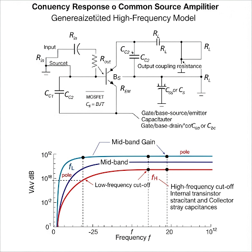
This section dives into the frequency response analysis relevant to common emitter (CE) and common source (CS) amplifiers, particularly considering the high-frequency models of BJTs and MOSFETs. It begins by introducing a generalized model consisting of input and output resistances, source capacitance, and coupling capacitors that affect the overall frequency response of the circuit.
The effective input and output capacitances are analyzed, specifically focusing on how they change with respect to the voltage gain of the amplifiers. Important parameters such as resistances and capacitances play a crucial role in defining the frequency response and determining the poles and zeros of the transfer function.
The analysis continues with a Laplace domain representation, yielding a transfer function that reveals the circuit's poles and the frequency behavior at low and high-frequency limits. For example, at very low frequencies, capacitors act as open circuits, leading to attenuation, while at mid-range frequencies, they permit signal flow, stabilizing gain. Finally, the section culminates in summing up the position of poles affecting the frequency response offering insights into the operational characteristics of the amplifiers in question.
Youtube Videos

Audio Book
Dive deep into the subject with an immersive audiobook experience.
Generalized Model of CE and CS Amplifiers
Chapter 1 of 6
🔒 Unlock Audio Chapter
Sign up and enroll to access the full audio experience
Chapter Content
Yeah. So, welcome after the break. So, we are talking about the, in fact, what we got it is the generalized model of CE and CS amplifier here. What it is having here it is the input signal source, having the source resistance of R, and then signal coupling capacitor C, and then if I consider this is the main amplifier where we do have the input resistance represented by this R1. And then we do have voltage dependent voltage source, which means that this is the core of the amplifier, then we do have the output resistance R2. And then C3 and C4, they are representing you know either Cπ, Cgs or Cgd based on whether the circuit it is CE amplifier or CS amplifier.
Detailed Explanation
In this chunk, we begin with the introduction to the generalized model for Common Emitter (CE) and Common Source (CS) amplifiers. It highlights the components of the model: the input signal source with resistance R, a coupling capacitor C, the main amplifier's input resistance R1, a voltage-dependent voltage source, and the output resistance R2. Capacitors C3 and C4 represent different parasitic capacitances, which vary depending on whether the configuration is a CE or CS amplifier. Understanding these elements is crucial for analyzing their frequency response.
Examples & Analogies
Think of the amplifier as a water system where R is like the water pipe's resistance to flow, and C is like a valve that controls how much water can pass through. Depending on how you configure the system (CE or CS), the way the water flows (or the signal propagates) will change, just as the amplifier's output will be affected by its design and components.
Capacitance Contribution to Input and Output
Chapter 2 of 6
🔒 Unlock Audio Chapter
Sign up and enroll to access the full audio experience
Chapter Content
So, this particular this capacitor it can be converted into two equivalent capacitance; one is for the input port, the other one is for the output port. And then, the input port part coming out of the C4 it is what we said is that C4-in or in this case A is equal to A_v. In fact, if you see here we are putting a ‒ sign here assuming that the polarity of the voltage dependent voltage source, here it is +ve. And on the other hand, so this is the contribution coming to the input port earlier we used to call C1. Now, let me put a different name C4; that means, the input port capacitance coming due to C4. So, likewise the output port capacitance coming due to C4, let you call this is C4-out.
Detailed Explanation
This chunk discusses how capacitor C4 in the amplifier circuit can be treated as contributing to two different equivalent capacitances: one for the input (C4-in) and another for the output (C4-out). The input capacitance is calculated by considering the gain of the amplifier (Av), leading to a relationship that modifies the input capacitance based on the properties of the dependent source in the circuit. Understanding this concept helps in analyzing how the frequency response is affected by these capacitances.
Examples & Analogies
Imagine you're trying to fill two buckets (input and output) using the same pipe (C4). Depending on how the pipe is configured, either bucket may fill up faster or slower, mimicking how input and output capacitances in an amplifier affect the signal processing.
Load Capacitance and Its Implications
Chapter 3 of 6
🔒 Unlock Audio Chapter
Sign up and enroll to access the full audio experience
Chapter Content
Yeah, I like to mention one thing here it is in the actual circuit CE amplifier or CS amplifier, typically we do have one DC decoupling capacitor or a AC coupling capacitor and typically used to name as C2. And then the C3 and C4 if I consider their typical magnitude, this may be in the order of say 10 µF whereas, the C4 may be in the range of say 100 pF. So, as a result the load coming at this node due to the series connection of C2 and C4 practically it is dominated by C4. So, that is why at this node or at this node whatever the effective load capacitance we do have coming out of say these two parts it is getting to be equivalent to C4.
Detailed Explanation
This piece emphasizes the importance of load capacitance in CE and CS amplifiers. The circuit typically includes a coupling capacitor (C2) and two other capacitors (C3 and C4). With C3 generally being much larger than C4, C4 dictates the effective load capacitance in the circuit. This information is crucial for understanding how load capacitance can influence the overall frequency response of the amplifier.
Examples & Analogies
Consider three different sized buckets being filled with water (C2, C3, and C4). If one bucket (C4) is much smaller than the others (like C2 and C3), it'll determine how quickly water drains from the system, much like how C4 influences signal transmission in the amplifier.
Frequency Response and Transfer Functions
Chapter 4 of 6
🔒 Unlock Audio Chapter
Sign up and enroll to access the full audio experience
Chapter Content
So, our first task is to find the frequency response from this point to this point, namely maybe in Laplace domain we can see, and then we can find what is the corresponding transfer function we are getting. So, in the next step, next slide what we are going to do? We are going to analyze this R series with C, in series with Rin.
Detailed Explanation
In this segment, the focus shifts to analyzing the circuit's frequency response using Laplace transform techniques. The objective is to compute the transfer function, which provides critical information about how the input signal is modified by the circuit. By analyzing the series connection of resistance (Rin) and capacitance (C), we can derive equations that describe how signals of different frequencies will be attenuated or amplified.
Examples & Analogies
Visualize tuning a guitar: adjusting the tension of the strings (like tuning parameters in the circuit) changes how each string vibrates, affecting the sound frequency output. Similarly, how we analyze and adjust R and C in the circuit will determine how the amplifier responds to different input signals.
Analyzing the Circuit for Frequency Response
Chapter 5 of 6
🔒 Unlock Audio Chapter
Sign up and enroll to access the full audio experience
Chapter Content
So, we do have this circuit, we do have R, and then C, and then R and the C coming in parallel. Now, if you see here to get the frequency response of this circuit namely in Laplace domain we can get the transfer function by considering this impedance which is R and then R in series with + R.
Detailed Explanation
In this section, the circuit under consideration is elaborated upon with focus on its layout. We have resistances and capacitances in a particular geometric configuration, potentially impacting how frequencies are processed. To obtain the frequency response, we derive a transfer function by examining the circuit's impedance using Laplace transforms. This allows us to express how the circuit alters the input signal based on frequency.
Examples & Analogies
Think of a team of workers (resistors) teaming up to get a job done (pass a signal). Depending on how they are organized (in series or parallel), the total amount of work done affects how quickly and effectively the job is completed. In our case, the impedance structure changes how signals are processed and transformed.
Numerical Example and Simplifications
Chapter 6 of 6
🔒 Unlock Audio Chapter
Sign up and enroll to access the full audio experience
Chapter Content
Now, let me consider a typical numerical value and based on that we make some assumption here. So, what we have here it is C which is a typically much smaller than C. So, probably we can ignore this part and then we can consider this term and then we can take C outside.
Detailed Explanation
In this part, practical numerical values are introduced to tailor the theoretical concepts. It is proposed that, since one capacitance C is much smaller than another, it can be neglected in calculations. This simplification is a common engineering practice to streamline analysis and focus on the most significant parameters affecting frequency response.
Examples & Analogies
Imagine packing a suitcase for a trip; if one item is very small compared to everything else, you might choose to leave it behind to save space and make packing easier. Similarly, in this circuit analysis, unimportant factors (like very small capacitance) can be overlooked when they don't significantly impact the results.
Key Concepts
-
Capacitance: Affects the frequency response by storing charge.
-
Poles: Determine system stability and frequency response characteristics.
-
Transfer Function: The mathematical formulation that relates output to input.
-
Attenuation: Describes how signals lose strength in circuits.
-
Frequency Response: Represents how the circuit handles different frequencies.
Examples & Applications
In a CE amplifier with a coupling capacitor of 10μF, as frequency increases, this capacitor progressively allows AC signals, influencing gain.
Using a Bode plot, the output of a CS amplifier can be analyzed to see how gain changes with frequency, noting poles at certain points.
Memory Aids
Interactive tools to help you remember key concepts
Rhymes
Capacitors at low, let signals go low, but in mid, they do show, how currents can flow.
Stories
Imagine a traffic light (capacitor) that lets cars (signals) flow at certain speeds (frequencies), stopping some at red (low frequencies) and clearing the road at green (mid frequencies).
Memory Tools
LSA - Low blocks, Stable allows.
Acronyms
P for Poles means Performance and Stability.
Flash Cards
Glossary
- Frequency Response
The output reaction of an electronic circuit to different input frequencies, analyzed typically in the frequency domain.
- Transfer Function
A mathematical representation of the output signal in relation to the input signal in the Laplace domain.
- Poles
Values of s in the transfer function that cause the output to become infinite; they significantly affect the system's stability and frequency response.
- Capacitance
Property of a circuit component that allows it to store an electric charge, influencing the frequency response.
- Attenuation
The reduction of signal strength as it passes through a medium.
Reference links
Supplementary resources to enhance your learning experience.