
Frequency Response Of CE/CS Amplifiers Considering High Frequency Models of BJT and MOSFET (Part C)
Enroll to start learning
You’ve not yet enrolled in this course. Please enroll for free to listen to audio lessons, classroom podcasts and take practice test.
Interactive Audio Lesson
Listen to a student-teacher conversation explaining the topic in a relatable way.
Understanding the Frequency Response
🔒 Unlock Audio Lesson
Sign up and enroll to listen to this audio lesson

Welcome everyone! Today, we are diving into the frequency response of common emitter and common source amplifiers. Can anyone tell me what 'frequency response' means?

It's how an amplifier responds to different frequencies of input signals.
Exactly! The frequency response is influenced by components like resistors and capacitors. What do you think happens at the extremes of high and low frequencies?

We might see attenuation or gain variations!
Correct! We use parameters like lower cutoff frequency to define where the response starts to drop off. Let's understand how to calculate this.
Calculating Cutoff Frequencies
🔒 Unlock Audio Lesson
Sign up and enroll to listen to this audio lesson

To calculate cutoff frequencies, we need to know the resistances and capacitances in our circuit. Can anyone remind us how to find the lower cutoff frequency based on resistance and capacitance?

Isn't it found using the formula fL = 1/(2πRC)?
Yes! Great job! Now, let's input some values: what happens if R = 650Ω and C = 10µF?

That would give us a lower cutoff frequency of about 8.16 Hz!
Right! Now let’s summarize this: the lower cutoff frequency indicates the frequency below which gain significantly falls off.
Mid-Frequency Gain Calculation
🔒 Unlock Audio Lesson
Sign up and enroll to listen to this audio lesson
Let’s discuss mid-frequency gain. Who can define what mid-frequency gain represents in our analysis?
It represents the typical gain of the amplifier in its optimal range.
Absolutely, and we can express this gain with the formula based on overall gain and attenuation factors. From our earlier example, what do we find for the mid-frequency gain?
It would be around -160 when considering the calculated attenuation!
Exactly! The negative sign indicates phase inversion. Always keep this in mind.
Real-World Applications of CE and CS Amplifiers
🔒 Unlock Audio Lesson
Sign up and enroll to listen to this audio lesson
Now let’s connect theory to real-world applications. How do you think engineers use these calculations when designing CE and CS amplifiers?
They likely ensure that amplifiers meet the required specifications for signal processing or audio applications.
Exactly! Understanding frequency response allows engineers to tailor designs to specific applications by selecting appropriate components.
Can we discuss how noise might affect these designs as well?
Sure! Noise can impact frequency response significantly; we shall explore that in future sessions!
Introduction & Overview
Read summaries of the section's main ideas at different levels of detail.
Quick Overview
Standard
This section elaborates on the frequency response of CE and CS amplifiers by applying high frequency models for BJTs and MOSFETs. Key concepts such as lower and upper cutoff frequencies, mid-frequency gain, and their calculations are explored through illustrative numerical examples, allowing students to understand real-world applications of these amplifiers.
Detailed
Detailed Summary
In this section, we delve into the frequency response of common emitter (CE) and common source (CS) amplifiers. We consider high frequency models of BJTs and MOSFETs to understand how signal characteristics evolve at different frequencies. The main aim is to evaluate the mid-frequency gain along with the lower and upper cutoff frequencies for these amplifiers.
We begin with a numerical example involving a CE amplifier with specified component values to calculate various frequency response parameters. We explore the equivalent circuit representation and detail the calculation of input capacitance, the first and second poles, and their relationship to cutoff frequencies. Furthermore, we analyze how the addition of capacitive elements affects the frequency response, culminating in a detailed exploration of gains and signal behaviors across these circuits.
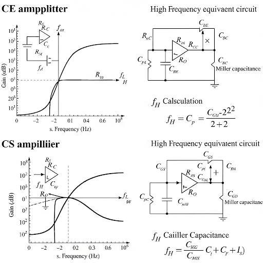
Finally, we extend the analysis to the CS amplifier, where similar principles are applied to derive frequency response characteristics. Through practical calculations and theoretical insights, this section serves as a knowledgeable foundation for understanding amplifier designs in analog electronics.
Youtube Videos

Audio Book
Dive deep into the subject with an immersive audiobook experience.
Introduction to Frequency Response
Chapter 1 of 7
🔒 Unlock Audio Chapter
Sign up and enroll to access the full audio experience
Chapter Content
Welcome back after the short break. So, we are going to discuss about numerical example, and the circuit it is still that equivalent circuit we do have and what we are. So, we do have the generalized equivalent circuit, but then also we do have additional information namely the value of different components, R this input resistance is 1.3 k, R output resistance it is a 3.3 k and then let you consider source resistance 650 Ω that is also a typical value one possible value of typical signal source.
Detailed Explanation
This chunk introduces the frequency response discussion and outlines the numerical example for analyzing CE (Common Emitter) and CS (Common Source) amplifiers. The essential circuit components are specified, such as input resistance (1.3 kΩ), output resistance (3.3 kΩ), and source resistance (650 Ω), which are crucial for frequency response calculations.
Examples & Analogies
Think of an amplifier as a water pipe system. Just as water pressure and resistance in pipes affect water flow, the resistances and capacitances affect the signal flow in amplifiers.
Capacitances in the Circuit
Chapter 2 of 7
🔒 Unlock Audio Chapter
Sign up and enroll to access the full audio experience
Chapter Content
And then the load capacitance C 100 pF, C it is given here it is say 10 µF and then C L which is one of the element contributing to input capacitance it is say 10 pF, C the Miller effected capacitance the capacitor which is breezing the input and output terminal of the circuit is 5 pF.
Detailed Explanation
In this chunk, several capacitances relevant to the amplifier circuit are listed, including load capacitance (100 pF), an additional capacitance of 10 µF (likely bypass capacitance), input capacitance (10 pF), and the Miller effect capacitance (5 pF). Understanding these capacitances is essential as they all impact the frequency response of the amplifier.
Examples & Analogies
Imagine using different sized balloons to hold water. Each balloon size changes how quickly water can flow. Similarly, different capacitances affect the speed of electrical signals in an amplifier circuit.
Calculating Frequency Response
Chapter 3 of 7
🔒 Unlock Audio Chapter
Sign up and enroll to access the full audio experience
Chapter Content
So, that means, actually this is ‒ and this is +. So, anyway with this information let we try to get the frequency response and particularly containing the mid frequency gain and then lower cutoff frequency and then upper cutoff frequency. So, how do we proceed?
Detailed Explanation
This segment transitions into calculating the frequency response, including the mid-frequency gain, lower cutoff frequency, and upper cutoff frequency. The overall method is to analyze how these frequencies can be affected by the previously mentioned resistances and capacitances.
Examples & Analogies
Consider tuning a musical instrument. To get the right sound (frequency), you need to adjust the tension of the strings (resistance) and their size (capacitance). The right adjustments provide the correct notes.
Lower Cutoff Frequency Calculation
Chapter 4 of 7
🔒 Unlock Audio Chapter
Sign up and enroll to access the full audio experience
Chapter Content
So, to start with let we calculate C and C = C (1 ‒ (‒240)), then + C . So, we do have here and then × 241 + 10. So, that gives us how much; we do have 1215, 1215 pF, yes.
Detailed Explanation
Here, we begin calculating the input capacitance (C_in) based on the contributions from the Miller effect and additional components. This calculation gives a value of 1215 pF, which will influence the frequency response regarding pole frequencies.
Examples & Analogies
It's like combining different weights to create an ideal balance for a scale. Each weight's contribution changes how the scale behaves, just like how capacitance change affects frequency response.
Second Pole Calculation
Chapter 5 of 7
🔒 Unlock Audio Chapter
Sign up and enroll to access the full audio experience
Chapter Content
So, we do have the C is given here, with this C we can calculate the location of the second pole and let we calculate the first pole first. So, p which is defined by if I express this in the unit of Hz then we have to consider 2π. So, 2π× , so this = . R it is 650 and then R , R it is 1.3 k, so that is 1950 this resistance and then C it is 10 µF which means 10‒5.
Detailed Explanation
In this step, the calculation of the first pole frequency (p1) is conducted using the resistances and capacitances of the circuit. By employing the formula involving 2π, the specific frequency values are determined, providing critical insights into the amplifier's operational limits.
Examples & Analogies
Think of a seesaw; the position and weight of each child affect how balanced the seesaw is. In electronics, poles determine how signals behave based on the circuit’s configurations.
Upper Cutoff Frequency Calculation
Chapter 6 of 7
🔒 Unlock Audio Chapter
Sign up and enroll to access the full audio experience
Chapter Content
And if you do this calculation what you will be getting it is 459, in my calculation that is what I obtain 459 kHz.
Detailed Explanation
The final pole calculation leads to finding the upper cutoff frequency, which is critical in defining the bandwidth of the amplifier. This value helps understand how quickly the amplifier can respond to frequency changes in the input signal.
Examples & Analogies
Consider the limits of a sports car’s speed; just like a car's top speed, the cutoff frequency tells you how fast the amplifier can respond to high-frequency signals.
Overall Frequency Response Summary
Chapter 7 of 7
🔒 Unlock Audio Chapter
Sign up and enroll to access the full audio experience
Chapter Content
So, in summary what we have so far we have covered it is. So, in this module what we have covered here it is basically we have considered high frequency model of transistor and particularly in presence of source resistance R, what is its impact on the frequency response of common emitter and common source amplifiers.
Detailed Explanation
This closing reflection points to the broader conclusions about frequency response in CE and CS amplifiers while emphasizing the effects of source resistance and how it shapes the amplifier’s performance. It wraps up the importance of understanding each component's contribution.
Examples & Analogies
Consider a recipe; all ingredients (like resistors and capacitors) must be harmonized for the dish (the amplifier's operation) to turn out well. Each component has a role in achieving the desired result.
Key Concepts
-
Frequency Response: Describes how amplifiers respond to different frequencies.
-
Cutoff Frequencies: Critical points defining the range over which an amplifier effectively operates.
-
Miller Effect: Affects input capacitance and frequency response due to feedback.
-
Pole Calculation: Key to assess frequency response characteristics.
Examples & Applications
If R = 1.3 kΩ and C = 10µF, the lower cutoff frequency can be calculated as fL = 1/(2πRC), yielding approximately 8.16 Hz.
For a common emitter amplifier with a mid-frequency gain of -240, the overall gain at mid frequencies can be adjusted based on loading effects.
Memory Aids
Interactive tools to help you remember key concepts
Rhymes
When frequencies low, gain will not show; but once at the right height, it gives quite a sight.
Stories
Imagine a musician tuning their guitar. When playing too low or too high, they lose notes, like an amplifier that drops gain at its cutoff frequencies.
Memory Tools
P-G-M: Pole-Gain-Miller to recall the key concepts of frequency responses.
Acronyms
F-R-C
Frequency Response Calculations
reminding you to consider how they behave in circuits.
Flash Cards
Glossary
- Common Emitter Amplifier
A type of BJT amplifier that provides high gain and inverts the input signal.
- Common Source Amplifier
A type of MOSFET amplifier similar to the CE amplifier but using a MOSFET instead of a BJT.
- Frequency Response
The output behavior of an amplifier across a range of frequencies.
- Cutoff Frequency
The frequency at which the output power falls to half its maximum value, typically defined as lower and upper cutoff frequencies.
- Miller Effect
A phenomenon in amplifiers where the input capacitance is increased by feedback through output capacitance.
- Poles
Specific frequencies in a system that define significant changes in amplitude or phase.
Reference links
Supplementary resources to enhance your learning experience.