
Kinematic equations for uniformly accelerated motion
Enroll to start learning
You’ve not yet enrolled in this course. Please enroll for free to listen to audio lessons, classroom podcasts and take practice test.
Interactive Audio Lesson
Listen to a student-teacher conversation explaining the topic in a relatable way.
Introduction to Kinematic Equations
🔒 Unlock Audio Lesson
Sign up and enroll to listen to this audio lesson

Today, we're going to learn about kinematic equations which allow us to connect the different variables in uniformly accelerated motion. Who can remind me what these variables are?

Is it displacement, time, initial velocity, final velocity, and acceleration?
Exactly! Each of these plays a crucial role in the equations we will discuss. Let's start with the first equation: v = v0 + at. Can anyone explain what this equation represents?

It shows how the final velocity depends on the initial velocity and acceleration over a certain time.
Great! This equation expresses how velocity changes with time when acceleration is constant. It's a foundation for understanding motion!

I remember 'v' stands for final velocity and 'v0' stands for initial velocity, but what does 'a' represent?
'a' represents acceleration. Let's summarize what we learned: the final velocity can be determined if we know the initial velocity, the acceleration, and how long the object accelerates.
Deriving Displacement Equations
🔒 Unlock Audio Lesson
Sign up and enroll to listen to this audio lesson

Now, let's dive into the displacement equations. We have x = v0t + (1/2)at². How do we arrive at this equation?

Isn't that from the area under the velocity-time graph?
Exactly! The area represents total displacement. This equation considers that the average velocity during constant acceleration is (v0 + v)/2. Can anyone calculate what the displacement is when acceleration is constant?
Is there a scenario that's a good example of this displacement?
Absolutely! An object dropped from a height, where its initial velocity is zero and moves under gravity, is a perfect example. This fascinates me; considering Earth's gravity gives us practical insight!
Practical Applications of Kinematic Equations
🔒 Unlock Audio Lesson
Sign up and enroll to listen to this audio lesson
How can we apply the kinematic equations in real-life situations? Any examples?
Like calculating how high a ball goes when thrown upward?
Exactly! And when we want to find out how long it takes to reach its peak height. We would use v = v0 + at while noting that at peak height, final velocity 'v' is zero.
Wait, can we also use these equations for cars stopping?
Great thought! You'd set 'v' as the final velocity when a car stops and work backwards to find stopping distance with v² = v0² + 2ax.
This seems so useful! Can we practice some example problems?
Absolutely! Let's summarize the equations next, then we'll dive into some real problems!
Introduction & Overview
Read summaries of the section's main ideas at different levels of detail.
Quick Overview
Standard
The section provides a comprehensive look at kinematic equations applied to uniformly accelerated motion, deriving formulas that relate displacement, initial velocity, final velocity, acceleration, and time. Key concepts include the significance of each equation and examples illustrating their application in problem-solving.
Detailed
Kinematic Equations for Uniformly Accelerated Motion
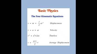
In this section, we explore the kinematic equations that govern the motion of objects under constant acceleration. These equations are crucial for understanding the basic principles of motion in physics. We derive formulas that relate the five key quantities: displacement (x), time taken (t), initial velocity (v0), final velocity (v), and acceleration (a).
Key Equations:
- Final Velocity equation:
v = v0 + at
- Displacement equations:
- Average method:
x = (v0 + v)t/2
- Rearranged for displacement:
x = v0t + (1/2)at²
- Relationship involving squares of velocities:
v² = v0² + 2ax
These equations allow us to analyze motion in a straightforward manner, enabling calculations of motion characteristics without needing to delve into the forces causing the motion. For example, the equation for displacement demonstrates how time influences how far an object travels when subjected to acceleration.
Importance:
The kinematic equations simplify the analysis of one-dimensional motion, making it easier to solve real-world problems using standard values for acceleration due to gravity, or different acceleration rates depending on the scenario. They have profound applications in not only physics but also various engineering fields.
Using these equations wisely not only helps in solving physics problems efficiently but also deepens the understanding of motion's nature.
Youtube Videos


Audio Book
Dive deep into the subject with an immersive audiobook experience.
Deriving Kinematic Equations
Chapter 1 of 6
🔒 Unlock Audio Chapter
Sign up and enroll to access the full audio experience
Chapter Content
For uniformly accelerated motion, we can derive some simple equations that relate displacement (x), time taken (t), initial velocity (v0), final velocity (v), and acceleration (a). Equation (2.4) already obtained gives a relation between final and initial velocities v and v0 of an object moving with uniform acceleration a:
v = v0 + at (2.4)
Detailed Explanation
In this chunk, we're introducing the basic kinematic equation that connects the final velocity (v) of an object to its initial velocity (v0), the acceleration (a), and the time taken (t). This formula is crucial because it allows us to predict the final speed of a moving object if we know how fast it started, the rate at which it accelerates, and how long it has been accelerating.
Examples & Analogies
Think about riding a bike. If you start at a certain speed and pedal hard, you accelerate (increase your speed). If you pedal for a certain time, you can figure out how fast you’ll be going at the end. If you start at 5 m/s and accelerate at 2 m/s² for 5 seconds, using this formula, you can find out that you’ll be going 15 m/s when you stop pedaling.
Understanding Displacement from Velocity
Chapter 2 of 6
🔒 Unlock Audio Chapter
Sign up and enroll to access the full audio experience
Chapter Content
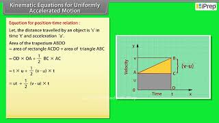
The area under this curve represents the displacement. Therefore, the displacement x of the object is:
( )1–20 0 x v v t + v t = (2.5)
Detailed Explanation
This chunk emphasizes that the area under the velocity-time graph (v-t graph) represents the object's total displacement during the time interval. This is because displacement is essentially how far the object has moved, and the area under the curve gives us a visual representation of that movement over time. It gives you not just the distance but also considers the velocity at which you were moving.
Examples & Analogies
Imagine you are driving a car and you see a graph showing how fast you're going over time. The area under that graph would represent how far you’ve traveled. If you speed up, the area grows bigger, showing that you covered more distance in less time.
Expressing Displacement with Average Velocity
Chapter 3 of 6
🔒 Unlock Audio Chapter
Sign up and enroll to access the full audio experience
Chapter Content
Equations (2.7a) and (2.7b) mean that the object has undergone displacement x with an average velocity equal to the arithmetic average of the initial and final velocities.
Detailed Explanation
This chunk explains two important equations that deal with displacement over time when an object is undergoing constant acceleration. The average velocity is computed by taking the average of the initial velocity (v0) and the final velocity (v). This makes sense because when an object accelerates uniformly, its speed doesn't just change instantly; it gradually increases, making the average velocity an important value to calculate displacement accurately.
Examples & Analogies
Imagine a runner in a race who starts slow but speeds up as they reach the finish line. To figure out their average speed for the entire race, you can take their starting speed and ending speed, average them, and then find out how far they ran in that time.
General Form of Kinematic Equations
Chapter 4 of 6
🔒 Unlock Audio Chapter
Sign up and enroll to access the full audio experience
Chapter Content
The set of Eq. (2.9a) were obtained by assuming that at t = 0, the position of the particle, x is 0. We can obtain a more general equation if we take the position coordinate at t = 0 as non-zero, say x0.
Detailed Explanation
Here, we shift focus from the specific case where the start position is set to zero. This chunk introduces the concept that we can account for scenarios where an object's position is not at zero when we start measuring time. By adjusting our equations to account for this initial position (x0), we can better analyze more complex situations where the object may not start from the origin.
Examples & Analogies
Think of someone dropping a ball from the top of a staircase. Instead of starting from zero height, they start from the height of the stairs (for example, 3 meters). By changing the starting point in our calculations, we can find out how far the ball falls regardless of where it starts.
Using Calculus to Derive Equations
Chapter 5 of 6
🔒 Unlock Audio Chapter
Sign up and enroll to access the full audio experience
Chapter Content
By definition, d/dt v = a; dv = a dt. Integrating both sides...
Detailed Explanation
In this chunk, we start using calculus to derive the equations of motion. We relate acceleration (a), which is the derivative of velocity (v) with respect to time (t). By integrating these relations, we can derive more precise equations that hold under various conditions for motion, including non-uniform motion. This approach provides a deeper mathematical understanding of how objects move.
Examples & Analogies
Picture painting a mural on a large wall. Each brushstroke (like a tiny change in position) works together over time to create a large picture. Calculus allows us to focus on those small pieces (tiny changes) that add up to understand the whole (the entire motion).
Applications of Kinematic Equations
Chapter 6 of 6
🔒 Unlock Audio Chapter
Sign up and enroll to access the full audio experience
Chapter Content
Now, we shall use these equations to some important cases. Example 2.3 discusses a ball thrown vertically upwards with a velocity of 20 m/s from 25.0 m high...
Detailed Explanation
This chunk introduces real-world examples of applying the kinematic equations we've derived. By looking at specific cases, such as a ball being thrown upwards, we can see how to apply these equations to find out how high the ball rises and how long it stays in the air before returning to the ground. It emphasizes that theory meets practice in practical scenarios.
Examples & Analogies
Imagine you throw a basketball upwards at the start of a game. You can calculate not just how high it goes, but also when it will come back down to your hands if you know the initial speed and the height from which you shot it.
Key Concepts
-
Kinematic Equations: Mathematical formulas linking displacement, velocity, and acceleration in uniformly accelerated motion.
-
Uniformly Accelerated Motion: Motion where an object's acceleration remains constant over time.
Examples & Applications
A ball thrown vertically up to its peak height demonstrates uniformly accelerated motion as it slows down due to gravity.
A car decelerating to a stop shows how the final velocity and stopping distance are calculated using kinematic equations.
Memory Aids
Interactive tools to help you remember key concepts
Rhymes
Velocity so steep, with time it will leap; acceleration's the key, to know where you'll be!
Stories
Once there was a car that had a constant acceleration, over time, it sped up further and further until it couldn't go faster; it learned its limits by measuring distance.
Memory Tools
To remember the kinematic equations: V = (V0 + A)T, X = (1/2)A(T^2), and V^2 = V0^2 + 2AX.
Acronyms
The acronym 'VAX' can remind you of Variables in kinematic equations
Velocity
Acceleration
eXit (displacement).
Flash Cards
Glossary
- Displacement
The change in position of an object, measured in meters.
- Velocity
The speed of an object in a particular direction.
- Acceleration
The rate of change of velocity of an object, measured in m/s².
- Kinematic Equations
Equations that describe the relationships between displacement, velocity, acceleration, and time.
Reference links
Supplementary resources to enhance your learning experience.