
Determination of Equilibrium Income in the Short Run
Enroll to start learning
You’ve not yet enrolled in this course. Please enroll for free to listen to audio lessons, classroom podcasts and take practice test.
Interactive Audio Lesson
Listen to a student-teacher conversation explaining the topic in a relatable way.
Understanding Macroeconomic Equilibrium Basics
🔒 Unlock Audio Lesson
Sign up and enroll to listen to this audio lesson

Welcome class! Today, we're diving into how we determine equilibrium income in a macroeconomic context. Can anyone summarize what equilibrium means in economic terms?

Equilibrium is when quantity demanded equals quantity supplied!
Exactly! In macroeconomics, we look at equilibrium in two stages. The first one considers the price level as fixed. Why do you think we start with a fixed price level?

Is it because we assume there are unused resources?
Great point! When there are unused resources, we can produce more without increasing costs. Remember this idea with the acronym 'SPUD'—S for Supply, P for Price level fixed, U for Unused resources, D for Demand.
Implications of Fixed Price Levels
🔒 Unlock Audio Lesson
Sign up and enroll to listen to this audio lesson

Now that we understand the fixed price assumption, how does it simplify our analysis?

It makes it easier to see how demand affects income levels without worrying about price changes.
Exactly! When analyzing this scenario, the law of diminishing returns does not apply, allowing us to focus solely on outputs. What would happen in reality if prices did vary while we were analyzing?

The equilibrium could change significantly as well, right?
Correct! This leads us to the second stage of our analysis. Let’s make sure we can summarize this; how would you say we approach equilibrium in the short run?
We first analyze with a fixed price level and then account for price changes.
Impact of Variable Price Levels
🔒 Unlock Audio Lesson
Sign up and enroll to listen to this audio lesson
Next, let’s explore how changes in price levels affect equilibrium income. What implications do you see from allowing prices to vary?
If prices go up, demand might decrease, affecting income.
Good observation! As prices increase, we can indeed see a shift. We should always remember to consider both supply and demand moving forward. Can anyone summarize the ‘fixed then flexible’ approach we’re analyzing?
We first look at a scenario with fixed prices to understand one facet of equilibrium before seeing how real-world price changes impact it.
Real-World Applications
🔒 Unlock Audio Lesson
Sign up and enroll to listen to this audio lesson
Let’s relate our learning to current events. Can anyone give an example where equilibrium shifts due to price level changes?
When the pandemic hit, some goods' prices increased, which shifted demand significantly!
Excellent example! It's crucial to see theory in action. How might economists react to such a shift in terms of policy?
They would need to adjust to either control inflation or stabilize income.
Well said! Remember, recognizing changes in equilibrium income is critical for effective policy-making in economics. Can you see how this all fits together?
Introduction & Overview
Read summaries of the section's main ideas at different levels of detail.
Quick Overview
Standard
The determination of equilibrium income involves two steps in macroeconomic theory. Initially, it considers a scenario with a fixed price level, assuming unused resources. This is followed by a broader analysis where price levels can change, exploring how this affects overall equilibrium.
Detailed
In macroeconomic theory, the equilibrium income is derived through two significant stages. In the first stage, the price level is considered fixed, which allows analysts to assume that additional output can be produced without any increase in marginal costs, due to the existence of unused resources such as machinery, buildings, and labor. This assumption simplifies the analysis and allows for a clear understanding of how demand and supply determine equilibrium income. In the second stage, the analysis incorporates variations in the price level, revealing how equilibrium can shift and adapt under different economic conditions. This structure aids in comprehending both short-term and long-term economic dynamics.
Youtube Videos


Audio Book
Dive deep into the subject with an immersive audiobook experience.
Understanding Macroeconomic Equilibrium
Chapter 1 of 10
🔒 Unlock Audio Chapter
Sign up and enroll to access the full audio experience
Chapter Content
You would recall that in microeconomic theory when we analyse the equilibrium of demand and supply in a single market, the demand and supply curves simultaneously determine the equilibrium price and the equilibrium quantity. In macroeconomic theory we proceed in two steps: at the first stage, we work out a macroeconomic equilibrium taking the price level as fixed. At the second stage, we allow the price level to vary and again, analyse macroeconomic equilibrium.
Detailed Explanation
In macroeconomics, the equilibrium of an economy is determined in two stages. First, we assume that the price level is constant, which allows us to analyze how total demand and total supply interact at that fixed price. Once we understand this interaction, we move to the second stage, where we allow prices to adjust and look for a new equilibrium. This approach contrasts with microeconomics, where demand and supply curves help find the equilibrium price and quantity simultaneously.
Examples & Analogies
Think of a market like a school fair. Initially, the prices of items are fixed (like ticket prices). You first see how many tickets students buy before adjusting prices based on supply and demand during the fair.
Justification for Fixed Price Level
Chapter 2 of 10
🔒 Unlock Audio Chapter
Sign up and enroll to access the full audio experience
Chapter Content
What is the justification for taking the price level as fixed? Two reasons can be put forward: (i) at the first stage, we are assuming an economy with unused resources: machineries, buildings and labours. In such a situation, the law of diminishing returns will not apply; hence additional output can be produced without increasing marginal cost. Accordingly, price level does not vary even if the quantity produced changes (ii) this is just a simplifying assumption which will be changed later.
Detailed Explanation
Taking the price level as fixed simplifies our analysis. First, if there are unused resources in the economy, we can increase output without raising costs – which means prices stay stable. Second, this assumption makes it easier to focus on understanding demand and supply interactions without complicating factors from price changes. Eventually, we'll factor in price changes to see how they affect equilibrium.
Examples & Analogies
Imagine a factory that has many machines sitting idle. If it produces more products without needing to hire new workers or buy new machines, it can keep prices of those products stable, making it easier to analyze how many products it sells based on buyers' demands.
Graphical Representation of Consumer Demand
Chapter 3 of 10
🔒 Unlock Audio Chapter
Sign up and enroll to access the full audio experience
Chapter Content
As already explained, the consumers demand can be expressed by the equation C=C+cY. Where C is Autonomous expenditure and c is the marginal propensity to consume.
Detailed Explanation
The consumer demand model shows how total consumption depends on autonomous expenditure (spending that occurs regardless of income) and the marginal propensity to consume (the fraction of additional income that is spent). If income increases, consumption also increases, reflecting the relationship outlined in the equation. This relationship can be visually represented in a graph which shows how changes in income affect total consumption.
Examples & Analogies
Imagine that someone gets a raise at work. Their base spending may always be the same (autonomous expenditure), but as they earn more, they also tend to spend a portion of that extra money on leisure or luxury items, illustrating how consumption rises with income.
Aggregate Demand Graphical Representation
Chapter 4 of 10
🔒 Unlock Audio Chapter
Sign up and enroll to access the full audio experience
Chapter Content
The Aggregate Demand function shows the total demand (made up of consumption + investment) at each level of income. Graphically it means the aggregate demand function can be obtained by vertically adding the consumption and investment function.
Detailed Explanation
Aggregate demand is the total demand in an economy at a given income level, reflecting combined consumer and investment spending. When we graph it, we can visualize how these two components interact. By stacking consumption and investment on a graph, the resulting function gives us a comprehensive picture of total demand across different income levels.
Examples & Analogies
Think of it like a pie chart divided into segments where each segment represents a different type of spending. The whole pie shows the total demand for goods and services in the economy, illustrating how much people want to buy at various income levels.
The 45-Degree Line: Supply Side of Equilibrium
Chapter 5 of 10
🔒 Unlock Audio Chapter
Sign up and enroll to access the full audio experience
Chapter Content
In the first stage of macroeconomic theory, we are taking the price level as fixed. Here, aggregate supply or the GDP is assumed to smoothly move up or down since they are unused resources of all types available. Whatever is the level of GDP, that much will be supplied and price level has no role to play. This kind of supply situation is shown by a 450 line.
Detailed Explanation
The 45-degree line graphical representation is essential for showing that every unit of GDP produced corresponds directly to the same amount supplied. Since we assume price remains fixed, as demand increases, production also increases along this line without affecting prices, indicating that the economy can respond to demand without constraints.
Examples & Analogies
It's like a factory that can scale up production indefinitely without costs changing, just like if every piece of equipment could produce exactly one more item for each additional worker hired, without any constraints or need to increase wages.
Equilibrium in Macroeconomics
Chapter 6 of 10
🔒 Unlock Audio Chapter
Sign up and enroll to access the full audio experience
Chapter Content
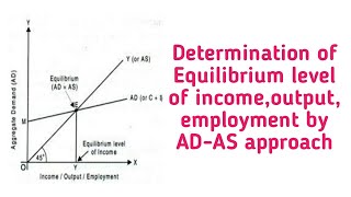
Equilibrium is shown graphically by putting ex ante aggregate demand and supply together in a diagram. The point where ex ante aggregate demand is equal to ex ante aggregate supply will be equilibrium.
Detailed Explanation
In macroeconomics, equilibrium occurs at the point where planned aggregate demand equals planned aggregate supply. When these two are equal, it indicates that the amount producers want to sell matches the amount consumers are willing to buy, meaning no excess supply or demand exists. This is crucial for understanding economic stability.
Examples & Analogies
Imagine a farmer and consumers at a market. If the farmer has exactly enough produce to meet what everyone wants to buy, that’s equilibrium. If the farmer has too much left over, he may need to lower prices to clear his goods. If he has too little, he could raise prices due to demand.
Algebraic Method for Finding Equilibrium
Chapter 7 of 10
🔒 Unlock Audio Chapter
Sign up and enroll to access the full audio experience
Chapter Content
Ex ante aggregate demand = I + C + cY. Ex ante aggregate supply = Y. Equilibrium requires that the plans of suppliers are matched by plans of those who provide final demands in the economy.
Detailed Explanation
To find equilibrium numerically, we set our equations for planned aggregate demand equal to those for planned supply. By solving for Y (output), we can find the income level where both supply and demand match. This algebraic approach offers a precise understanding of how variables interact and reveal the economy's behavior.
Examples & Analogies
Think of it like planning a school event where the number of attendees you expect must match the number of seats prepared. You check your number calculations carefully to ensure that every seat is filled – that’s how equilibrium is achieved in the economy.
Effect of Autonomous Changes on Income
Chapter 8 of 10
🔒 Unlock Audio Chapter
Sign up and enroll to access the full audio experience
Chapter Content
We have seen that the equilibrium level of income depends on aggregate demand. Thus, if aggregate demand changes, the equilibrium level of income changes.
Detailed Explanation
Equilibrium income is sensitive to changes in aggregate demand. If, for example, consumer spending or investment increases, it can shift the aggregate demand curve. As a result, equilibrium income will rise, reflecting more activity in the economy. Understanding this relationship helps economists predict economic fluctuations and plan fiscal policies.
Examples & Analogies
It’s like adjusting your budget for a family trip: if you decide to go to a more expensive restaurant, your overall spending must adjust, potentially shifting funds from other activities. Similarly, in the economy, a shift in spending changes overall income levels.
The Multiplier Mechanism Explained
Chapter 9 of 10
🔒 Unlock Audio Chapter
Sign up and enroll to access the full audio experience
Chapter Content
The production of final goods employs factors such as labour, capital, land and entrepreneurship. In the absence of indirect taxes or subsidies, the total value of the final goods output is distributed among different factors of production – wages to labour, interest to capital, rent to land etc.
Detailed Explanation
The multiplier effect illustrates how initial changes in spending lead to greater overall shifts in income and spending in the economy. As businesses produce more due to increased demand, they hire more labor, pay wages, and create a cycle where increased income further boosts consumption and demand in subsequent rounds. Essentially, every round of spending creates further economic activity.
Examples & Analogies
Imagine a pebble being dropped into a pond. The initial splash is like an increase in spending, and the ripples that move outwards represent increased economic activity as the initial spending leads to more jobs, higher wages, and further spending.
Understanding the Paradox of Thrift
Chapter 10 of 10
🔒 Unlock Audio Chapter
Sign up and enroll to access the full audio experience
Chapter Content
If all the people of the economy increase the proportion of income they save...the total value of savings in the economy will not increase – it will either decline or remain unchanged.
Detailed Explanation
The Paradox of Thrift reveals a counterintuitive concept: if everyone tries to save more money at once, it can actually lead to lower total savings in the economy. As people save more, they spend less, leading to decreased demand for goods and services. This reduction can result in lower income for workers, which in turn causes total savings to decrease as consumers have less income to save. It's a cycle that demonstrates that savings behavior must be balanced with consumption.
Examples & Analogies
Think of a community deciding to save for a new park by not spending on local businesses. If everyone reduces their spending, businesses earn less, which could lead to lower wages or layoffs, eventually meaning there’s less money to save. So their total savings might actually drop despite their intention to save more.
Key Concepts
-
Fixed Price Level: An assumption in the first stage where prices do not change, allowing analysis of production without adding costs.
-
Unused Resources: Resources not actively in use, which can affect production capacity.
-
Macroeconomic Equilibrium: The interaction of aggregated supply and demand to determine overall economy performance.
Examples & Applications
If an economy has high unemployment, there are many unused resources, meaning production can increase without affecting prices initially.
In times of inflation, rising prices may decrease demand, affecting overall income and output levels.
Memory Aids
Interactive tools to help you remember key concepts
Rhymes
To fix or not to fix, that's the question, resources sit idle, avoid dispossession.
Stories
Once upon a time in an idle economy, resources waited for demand to cause harmony in production.
Memory Tools
SPUD: Supply in equilibrium, Price level fixed, Unused resources grow, Demand seated.
Acronyms
EIRS
Equilibrium Income
Reaches Supply.
Flash Cards
Glossary
- Equilibrium
A state where economic forces such as supply and demand are balanced.
- Macroeconomic Equilibrium
The overall balance achieved in the economy when all markets are in equilibrium simultaneously.
- Price Level
An index that tracks the average level of prices in the economy.
- Unused Resources
Assets, such as labor and machinery, that are available but not being utilized in production.
- Law of Diminishing Returns
A theory that states that adding more of one factor of production, while keeping others constant, will eventually yield lower per-unit returns.
Reference links
Supplementary resources to enhance your learning experience.