
Example of PID Control Design
Enroll to start learning
You’ve not yet enrolled in this course. Please enroll for free to listen to audio lessons, classroom podcasts and take practice test.
Interactive Audio Lesson
Listen to a student-teacher conversation explaining the topic in a relatable way.
Analyzing the System Dynamics
🔒 Unlock Audio Lesson
Sign up and enroll to listen to this audio lesson

To begin our PID controller design, we need to analyze the system dynamics using its transfer function, G(s) = 10/(s² + 3s + 10). This function helps us identify key characteristics like the natural frequency and damping ratio.

Why are the natural frequency and damping ratio so important?
Great question! The natural frequency helps us understand how quickly the system reacts, while the damping ratio indicates how oscillatory the system might be. Together, they guide our PID tuning choices.

Can we calculate them directly from the transfer function?
Yes, you can! For second-order systems, these can be derived directly from the coefficients in the transfer function. Understanding these helps ensure our system remains stable.

So, if we set the Kp too high, that might destabilize the system?
Exactly! If Kp is too high, it could lead to overshoot or even oscillations, which can be detrimental to our system's performance.

And that’s why we need to analyze the system first?
Precisely! Analyzing the system gives us the foundation for designing an effective PID controller. Let's move on to selecting the PID parameters.
Selecting PID Parameters
🔒 Unlock Audio Lesson
Sign up and enroll to listen to this audio lesson

Now that we understand the dynamics, let's discuss how we select the PID parameters. Common methods include the Ziegler-Nichols tuning method and manual tuning approaches.
What is the Ziegler-Nichols method, and how does it work?
The Ziegler-Nichols method starts by setting both Ki and Kd to zero, then increasing Kp until we observe sustained oscillations. This helps find our critical gain, Ku, essential for determining the PID parameters.
What should we do after we find Ku?
We can then calculate Kp, Ki, and Kd based on the observed oscillation period. It's an empirical procedure but often produces a good starting point for fine-tuning.
If we use manual tuning, what should we consider?
Manual tuning involves adjusting the parameters while observing system responses, which can be handy for simpler systems or when a model is not available.
And is there a downside to manual tuning?
Yes, it can be time-consuming and less precise. However, with practice, many engineers find it effective in real-world scenarios. Let’s simulate the system response next.
Simulating the System Response
🔒 Unlock Audio Lesson
Sign up and enroll to listen to this audio lesson
Simulation plays a critical role in our PID design process. Once we select the parameters, we use tools like MATLAB or Python to model the system's response to a step input.
What are we looking for in the simulation?
We aim to observe how well the system achieves the desired temperature with minimal overshoot and acceptable settling time. Evaluating these responses guides further adjustments.
What if the overshoot is too large?
If overshoot is too high, we may need to lower Kp or increase Kd to dampen the response. The simulation helps us make those decisions without risking the physical system.
Can we also visualize the steady-state error?
Absolutely! It’s essential to check if the steady-state error is driven to zero, indicating adequate performance of our PID controller. Carefully analyze the response curve!
Got it! And after simulation, we adjust our settings?
Exactly! Simulation helps ensure a smoother design process. Let’s summarize what we’ve covered.
Adjusting PID Parameters
🔒 Unlock Audio Lesson
Sign up and enroll to listen to this audio lesson
After simulation, we evaluate our results, looking specifically at overshoot, settling time, and steady-state error. Adjusting the PID parameters helps refine performance.
So it’s crucial to iterate between simulation and adjustments?
Yes! It’s an iterative process. Based on the simulation results, we may need to tweak Kp, Ki, or Kd to meet specified performance metrics.
What happens if adjustments don’t improve the response?
If adjustments don’t yield improvements, it might be beneficial to revisit our system analysis to ensure the parameters we’re trying to tune align with the physical system’s behavior.
Can we lock in parameters once we’re satisfied?
Yes! Once satisfied with the controller performance, you can lock in those parameters and implement them in the actual system. Strong simulations validate our approach.
Awesome! This makes PID controller design feel much more approachable.
It definitely is! With careful tuning and refinement, PID controllers can greatly enhance system performance. Remember to follow the steps we've discussed as you design your own controllers!
Introduction & Overview
Read summaries of the section's main ideas at different levels of detail.
Quick Overview
Standard
The section outlines a step-by-step procedure for designing a PID controller tailored to a given heating system's transfer function. Key aspects covered include analyzing system dynamics, selecting PID parameters, simulating system response, and adjusting parameters to meet specific performance criteria.
Detailed
Example of PID Control Design
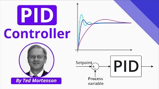
In this section, we explore a practical example of designing a PID controller for a heating system to maintain a constant temperature. The PID (Proportional-Integral-Derivative) controller is vital for dynamic control, as it helps achieve specified performance goals like minimal overshoot and suitable settling time.
Key Points:
- Analyze the System Dynamics: First, we derive the natural frequency and damping ratio using the system's transfer function represented by G(s) = 10/(s² + 3s + 10). This analysis helps understand the system's response characteristics.
- Select PID Parameters: Utilizing tuning methods such as the Ziegler-Nichols method, we determine initial values for the proportional (Kp), integral (Ki), and derivative (Kd) gains based on system behavior.
- Simulate the Response: Next, we employ simulation tools (e.g., MATLAB, Python) to observe how well the PID controller manages the system when subjected to a step input, particularly looking for characteristics like overshoot and settling time.
- Adjust the PID Parameters: Finally, based on the simulation outcomes, adjustments to the PID controller parameters are made to ensure that the system responds appropriately to disturbances while minimizing overshoot and eliminating steady-state errors.
Through these steps, the design of an effective PID controller can be achieved, showcasing the real-world applications of PID control in engineering.
Youtube Videos
Audio Book
Dive deep into the subject with an immersive audiobook experience.
Problem Statement
Chapter 1 of 5
🔒 Unlock Audio Chapter
Sign up and enroll to access the full audio experience
Chapter Content
Example Problem: Design a PID controller for a heating system.
Given:
● The transfer function of the system is G(s)=10s^2+3s+10.
● The system is required to heat a room and maintain a constant temperature, responding to a step input with minimal overshoot and settling time.
Detailed Explanation
This section introduces a practical example in which we are tasked with designing a PID controller for a heating system. The problem states that we have a transfer function, G(s), which is a mathematical representation of how well our system responds to inputs, in this case, heating a room. The objective is to design the PID controller so that when a step input (a sudden change in temperature requirement) is applied, the heating system maintains a constant temperature with minimal overshoot (going too high above the desired temperature) and settling time (the time it takes to reach and stabilize at the desired temperature).
Examples & Analogies
Imagine you are adjusting the temperature of your home using a thermostat. If you set the thermostat to 70°F and the current temperature is 65°F, your heating system needs to increase the temperature quickly while avoiding going past 70°F. The PID controller helps in achieving that balance, ensuring the room heats up effectively without getting too hot.
System Dynamics Analysis
Chapter 2 of 5
🔒 Unlock Audio Chapter
Sign up and enroll to access the full audio experience
Chapter Content
- Analyze the system dynamics:
○ Using the system’s transfer function, we identify the natural frequency and damping ratio of the system.
Detailed Explanation
In the first step of the design process, we analyze the system's dynamics based on the given transfer function, G(s). This usually involves identifying crucial characteristics of the system, such as the natural frequency, which indicates how quickly the system can respond to changes, and the damping ratio, which tells us about the stability and oscillation behavior of the system. These parameters are essential for tuning the PID controller effectively to achieve the desired performance.
Examples & Analogies
Think of riding a bicycle. The natural frequency would relate to how quickly the bike responds to your steering, while the damping ratio would be similar to how easily the bike settles after going over bumps. For our heating system, finding these factors helps us understand how 'nervous' or 'calm' our system is when reacting to changes in temperature.
Selecting PID Parameters
Chapter 3 of 5
🔒 Unlock Audio Chapter
Sign up and enroll to access the full audio experience
Chapter Content
- Select PID parameters:
○ Apply the Ziegler-Nichols method or manual tuning to set the values of Kp, Ki, and Kd.
Detailed Explanation
Once we understand the dynamics of the heating system, we need to select appropriate values for the PID controller's parameters: Kp (proportional gain), Ki (integral gain), and Kd (derivative gain). The Ziegler-Nichols method is a widely used technique that helps in determining these values based on system response. Alternatively, manual tuning allows us to adjust these parameters by observing the system's behavior directly and making changes until we achieve the desired performance.
Examples & Analogies
This step is like cooking a dish where you have to adjust ingredients by taste. You begin with a base recipe (the Ziegler-Nichols method) but must tweak the amounts based on how the dish tastes (manual tuning). Finding the right balance of ingredients can make your dish just perfect, similar to fine-tuning PID settings for optimal heating control.
Simulating the Response
Chapter 4 of 5
🔒 Unlock Audio Chapter
Sign up and enroll to access the full audio experience
Chapter Content
- Simulate the response:
○ Use tools like MATLAB or Python to simulate the system response to a step input with the PID controller.
Detailed Explanation
In this step, we utilize simulation tools like MATLAB or Python to model how the PID controller will perform with the chosen parameters when faced with a step input. This simulation allows us to visualize how quickly and effectively the heating system reaches the target temperature, along with its overshoot and settling behavior, giving us insights into whether our parameters need adjustments.
Examples & Analogies
Imagine testing a new recipe in your kitchen before serving it to guests. You take notes as you adjust the heat and timing to see how close you can get to the perfect meal. Similarly, in our heating system design, running simulations helps us 'taste-test' and refine our PID controller before it goes live in real situations.
Adjusting PID Parameters
Chapter 5 of 5
🔒 Unlock Audio Chapter
Sign up and enroll to access the full audio experience
Chapter Content
- Adjust the PID parameters:
○ Refine the controller parameters to reduce overshoot, improve settling time, and eliminate steady-state error.
Detailed Explanation
After simulating the system's response, we may find areas for improvement, such as excessive overshoot (where the temperature goes beyond the target) or long settling times (when it takes too long to stabilize at the target). This step involves tweaking the values of Kp, Ki, and Kd based on simulation results and iterating until we achieve a satisfactory performance, ensuring the system effectively responds to temperature changes without erratic behavior.
Examples & Analogies
Think of fine-tuning a musical instrument. After playing, you listen carefully (simulation) and notice it’s slightly off-key (overshoot or settling time). You adjust the tuning pegs (PID parameters) to bring it back to harmony. Just as you want beautiful music, we want our heating system to reach and maintain the desired temperature as seamlessly as possible.
Key Concepts
-
PID Controller Design: The process of designing a PID controller involves systematic analysis, parameter selection, simulation, and iterative adjustments.
-
Transfer Function: A mathematical model that defines the input-output relationship of the system.
-
Natural Frequency: A vital characteristic that indicates the system's responsiveness.
-
Damping Ratio: A crucial parameter that affects the stability and oscillatory behavior of the system.
Examples & Applications
One practical example discussed is designing a PID controller for a heating system with a given transfer function, G(s) = 10/(s² + 3s + 10).
Another example involves simulating the system's response to a step input and adjusting PID parameters based on observed overshoot and settling time.
Memory Aids
Interactive tools to help you remember key concepts
Rhymes
PID is three, with components key, Proportional, Integral, and Derivative, you see!
Stories
Imagine a temperature controller in a bakery. It uses PID to keep the oven’s heat just right—balancing how hot it is with how it’s warming up, ensuring perfect cakes every time!
Memory Tools
To remember the PID sequence, think ‘Pasta In Delight’ - Proportional, Integral, Derivative.
Acronyms
PID
Proportional
Integral
Derivative - remember it as 'Pride in Design'.
Flash Cards
Glossary
- PID Controller
A control mechanism that utilizes Proportional, Integral, and Derivative components to minimize error and improve system control.
- Transfer Function
A mathematical representation of a system's output in relation to its input, typically expressed in the s-domain.
- Natural Frequency
The frequency at which the system would oscillate if not subjected to damping.
- Damping Ratio
A measure of how oscillations in a system decay after a disturbance, affecting the system's stability.
Reference links
Supplementary resources to enhance your learning experience.