
Horizontal Water Jet Impact Problem
Enroll to start learning
You’ve not yet enrolled in this course. Please enroll for free to listen to audio lessons, classroom podcasts and take practice test.
Interactive Audio Lesson
Listen to a student-teacher conversation explaining the topic in a relatable way.
Understanding Momentum Flux Correction Factor
🔒 Unlock Audio Lesson
Sign up and enroll to listen to this audio lesson

Today, we are diving into the concept of momentum flux correction factors, especially under different flow conditions such as laminar and turbulent flows. Who can tell me what the term 'momentum flux' refers to?

Is it the amount of momentum flowing through a surface per time unit?
Exactly! Now, in laminar flow, we often find that this requires a modification termed the 'beta factor.' Does anyone remember what the common value of the beta factor is for laminar flows?

Is it one-third?
Correct! So when we calculate momentum flux under laminar conditions, it’s one-third of what we would typically expect. This helps us better model the force acting on surfaces. Now, can anyone explain why this is different for turbulent flow?

In turbulent flow, the velocity distribution is more uniform, so the beta factor is close to 1?
Exactly right! This change is crucial in practical engineering problems.
In summary, understanding the correction factor not only helps us predict the actual behavior of the fluid but also informs design and safety measures in engineering contexts.
Application of Momentum Flux in Practical Problems
🔒 Unlock Audio Lesson
Sign up and enroll to listen to this audio lesson

Let’s apply what we’ve learned to a practical example involving a sluice gate. Can someone describe how to approach this kind of problem?

We would first look at how fluid flow goes into and out of the gate, right?
Exactly! When analyzing the flow into the sluice gate, we’ll always consider mass conservation principles. Who can tell me how we might establish a formula for this?
We can equate the inflow and outflow rates while considering the head pressures at each side.
Correct! And these pressures will incorporate our earlier discussion about the momentum flux correction factors. By using the calculated head heights and velocities, we can solve for the force on the gate. Can anyone suggest what factors influence that force?
The velocities, height of the water, and the density!
Perfect! Applying these values allows us to compute the total force efficiently.
Solving Example Problems
🔒 Unlock Audio Lesson
Sign up and enroll to listen to this audio lesson
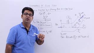
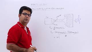
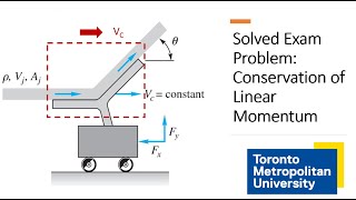
Let's consider a horizontal water jet striking a flat plate. We need to determine the total force acting on this plate given certain variables. How do we start?
We would begin by identifying the given information, like the velocity of the jet and its cross-sectional area.
Exactly! With the velocity at 10 m/s and the area at 10 mm², we can calculate flow rate. What unit conversions would we need to perform?
Convert the area from mm² to m²!
Correct. After calculating the flow rate, we can apply the momentum principle and derive the impact force. Can anyone calculate the expected force?
Using the momentum flux equals the density times velocity times area, right? So that gives us a clear way to find the force!
Excellent! This is the essence of applying theoretical fluid mechanics concepts with practical engineering scenarios to derive significant results.
Introduction & Overview
Read summaries of the section's main ideas at different levels of detail.
Quick Overview
Standard
The section elaborates on the application of momentum flux correction factors when analyzing the impact of horizontal water jets on flat plates. It highlights the relationships between velocity distributions and momentum flux, emphasizing how laminar and turbulent flows differ in their effect on calculations.
Detailed
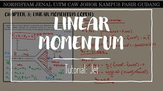
Horizontal Water Jet Impact Problem
This section delves into the critical analysis of horizontal water jet impacts, particularly how momentum flux and its correction factors play significant roles in fluid mechanics. Initially, the section explores the derivation of relationships governing momentum flux across various conditions, with a particular focus on laminar and turbulent flows.
Key points include the importance of velocity distribution in calculating momentum flux. In uniform flow, velocity distributions can yield larger momentum flux calculations, while non-uniform distributions, as seen in laminar flows, necessitate adjustments expressed through the beta factor, which is notably one third in laminar conditions. The implications of this adjustment help students understand how to compute real-world forces acting on structures subjected to fluid flows, exemplified through computational problems involving sluice gates and water jets.
The section provides practical examples that demonstrate how to derive forces acting on flat plates held normal to the flow direction, analyzing variables such as flow depth, velocities, and density. This thorough examination underscores how momentum conservation and mass balance principles apply in real-world engineering scenarios of fluid dynamics.
Youtube Videos


Audio Book
Dive deep into the subject with an immersive audiobook experience.
Momentum Flux Correction Factors
Chapter 1 of 6
🔒 Unlock Audio Chapter
Sign up and enroll to access the full audio experience
Chapter Content
And once I know this area and once I apply these things to the momentum flux correction factor equations, I will have a this far.
To do these integrations, we can consider and in terms of y we are writing it to just do the integrations, nothing else. In that, if you look it, you have y = 1 @ r = 0 and y = 0 @ r = R. So we will change this upper limit and lower limit of the equations when we are converting from dr to the y integrations. So, this is what, 0 to 1, the -1 components are there, -y square will be there. And if you substitute these values, and you will get it one by third. So, in laminar flow case whatever this velocity distributions, the beta factor is called, comes to what one by third.
Detailed Explanation
The passage discusses the calculation of momentum flux correction factors, which are important when dealing with laminar flow. It explains that upon integration, the variable y must change limits within the equations based on the position in the flow (from 0 to 1). The results indicate that for laminar flow, the moment flux correction factor (beta) is typically 1/3, meaning that when using average velocities in computations, the actual momentum flux through the surface is only one-third of that predicted by average values. This highlights the significance of proper velocity distribution recognition in fluid dynamics.
Examples & Analogies
Think of it like measuring the speed of a runner in a marathon. If you only look at the average speed for all runners without considering the different pacing strategies they use (some sprint, some walk, etc.), you might miscalculate how fast a runner might actually be going at different moments. The same applies here; the flow isn't uniform, and average calculations can lead to misunderstandings.
Understanding Pressure and Velocity Distribution
Chapter 2 of 6
🔒 Unlock Audio Chapter
Sign up and enroll to access the full audio experience
Chapter Content
What it indicates that the momentum flux using velocity distributions divide by the momentum flux using average velocity. So, what it indicates that, the momentum flux using the velocity distribution will be the one third of the momentum flux using average velocity. The momentum velocity using the average velocity is much, much larger and that what is to be divide by one third to compute it the momentum flux using the velocity distribution.
Detailed Explanation
This chunk explains that there’s a critical difference between momentum flux calculated with a uniform average velocity and that calculated with an actual velocity distribution. In scenarios where flow is not uniform (like in a jet stream), the actual momentum flux is significantly lower when you categorize it based on real flow characteristics. This is crucial for accurate engineering calculations involving fluid mechanics.
Examples & Analogies
Imagine a crowded subway where each person walks at different speeds. If you were to calculate how quickly they are moving on average during peak hours, you'd find your numbers don’t reflect the reality of individual speeds. This is similar to how fluid momentum must consider realistic distributions rather than simple averages.
Application of Forces on a Sluice Gate
Chapter 3 of 6
🔒 Unlock Audio Chapter
Sign up and enroll to access the full audio experience
Chapter Content
Now, let us come to the second example, which is very interesting example, which is almost all the Fluid Mechanics book have these examples with some numerical values are the difference. The problem is very interesting problems is that, there is a gate and the flow is coming from this side and going out through the gate here, the velocities V1 and V2 and h1 and h2 is the flow depth, this is the sluice gate.
To compute the forces acting on the gate, we derive a formula using inlet and outlet conditions and then substitute numerical values for precise calculations.
Detailed Explanation
This portion introduces a practical fluid mechanics problem dealing with a sluice gate, which controls the flow of water. It states that we must derive a formula for the force required to keep the gate shut against incoming water, taking into account velocity (V1 and V2) and flow depths (h1 and h2). Understanding these parameters allows for an accurate calculation of the total force on the gate, incorporating hydrostatic pressure and velocity changes.
Examples & Analogies
Think about holding back a garden hose with your hand. The faster the water flows through it, the more pressure you feel behind your hand. Similarly, the sluice gate experiences forces stemming from the pressure of flowing water that must be calculated to ensure it is secured properly against the flow.
Mass Conservation in Fluid Flow
Chapter 4 of 6
🔒 Unlock Audio Chapter
Sign up and enroll to access the full audio experience
Chapter Content
Now if you look it, I will apply mass conservation equation, because is single inlet and outlet conditions, the mass influx is equal to mass outflux, is a very simple problem, Outflow = Inflow. Incompressible flow.
Detailed Explanation
The principle of mass conservation states that mass must be conserved in a closed system. In this case, when working with flow through a sluice gate, the mass entering through one side must equal the mass exiting through the other side. This idea underpins various calculations in fluid dynamics, as it allows us to set equations based on flows maintained in a steady state.
Examples & Analogies
Picture a funnel: when you pour liquid into a funnel, the volume of liquid going in should equal the volume coming out at the bottom. But if you pour too quickly, it might overflow; similarly, if the inlet and outlet relationships through the sluice gate are not maintained, issues may occur in the flow.
Velocity and Pressure Distribution Impact
Chapter 5 of 6
🔒 Unlock Audio Chapter
Sign up and enroll to access the full audio experience
Chapter Content
Now, first is pressure distribution. Now, if this is my control volume, first I need to draw the streamlines. So, as it expected that the streamlines will be like this, so as actual fluid valve if you have it could be like this. The velocity distributions will come like this. So, you have a uniform velocity distribution what is assumption is there and make it a uniform velocity value.
Detailed Explanation
This segment discusses how streamlines help us visualize the flow and pressure distribution in fluid mechanics. Drawing streamlines enables us to anticipate how pressure varies across the control volume where the gate is located. Understanding how velocities change and distribute within that flow helps predict how forces will act on structures like gates.
Examples & Analogies
Imagine watching traffic flow on a highway. Some cars move faster than others, but you can see where the congestion happens. This is similar to how we must visualize and understand fluid movement to correctly manage how water will behave against physical barriers.
Forces Acting on the Jet
Chapter 6 of 6
🔒 Unlock Audio Chapter
Sign up and enroll to access the full audio experience
Chapter Content
Now that we have to look at the velocity distributions, there will be a shear stress acting on this. Because of this shear stress, there will be the force, but since here, the force due to the pressure distributions and momentum flux, rate of change of the momentum flux are much, much higher order, than force due to shear stress. So, we can neglect it, as compared to the pressure and momentum force component concept.
Detailed Explanation
This chunk highlights the forces arising from shear stress, pressure distributions, and momentum flux in fluids. While shear stress does exert some influence, it is generally negligible compared to the larger forces created by pressure and changes in momentum as water velocity varies near surfaces.
Examples & Analogies
Think of a bowling ball rolling on a smooth surface. The friction (shear stress) between the ball and the surface is minimal compared to the force of gravity pulling it down. In a similar manner, the overwhelming forces at play in fluid dynamics often dwarf the effects of minor forces like shear.
Key Concepts
-
Momentum Flux: Measures momentum flow rate across surfaces.
-
Beta Factor: Represents the correction needed for non-uniform velocity distributions.
-
Laminar vs Turbulent Flow: Differentiates flow pattern types which influence practical calculations.
-
Control Volume Analysis: An approach to apply mass and momentum conservation principles in fluid dynamics.
Examples & Applications
Example 1: Calculating the force on a sluice gate considering depth and velocity.
Example 2: Determining impact force from a horizontal water jet based on velocity and area.
Memory Aids
Interactive tools to help you remember key concepts
Rhymes
In laminar flows, it’s clear and slow, one-third is where the beta will go!
Stories
Imagine a calm river flowing smoothly, that’s laminar. Now picture a busy waterfall—chaotic! That’s turbulent flow!
Memory Tools
Lambda for Laminar, Turbo for Turbulent! Remember: L comes before T for lower to higher.
Acronyms
FLUID
Force
Laminar
Uniform
Impact
Density.
Flash Cards
Glossary
- Momentum Flux
The quantity of momentum transferred through a surface per unit time.
- Beta Factor
A correction factor used in fluid mechanics to account for changes in velocity distribution.
- Laminar Flow
A type of flow in which fluid moves in parallel layers with minimal disruption.
- Turbulent Flow
A type of flow characterized by chaotic changes in pressure and velocity.
- Hydrostatic Pressure
The pressure exerted by a fluid at rest due to its weight.
- Control Volume
A defined volume in space through which fluid flows for analysis.
Reference links
Supplementary resources to enhance your learning experience.