Laminar and turbulent flow (Cond.)
Enroll to start learning
You’ve not yet enrolled in this course. Please enroll for free to listen to audio lessons, classroom podcasts and take practice test.
Interactive Audio Lesson
Listen to a student-teacher conversation explaining the topic in a relatable way.
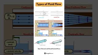
Laminar Flow Basics
🔒 Unlock Audio Lesson
Sign up and enroll to listen to this audio lesson

Today, we will discuss laminar flow. Can anyone tell me what laminar flow is?

Isn't it when the fluid flows in parallel layers?

Exactly! Laminar flow occurs when fluid moves in smooth layers with minimal disturbance. What defines the maximum velocity in this scenario?

I think it has to do with the viscosity and pressure gradient, right?

Correct! The maximum velocity can be calculated using the formula derived from the flow equations. For laminar flow between two plates, the maximum velocity, U_max, can be determined using U_max = -1/8 * (mu * dp/dx * t^2).

And what about the shear stress at the wall?

Good question! The shear stress, tau_0, at the wall can be calculated using the formula tau_0 = mu * du/dy at y = 0. Remember, tau_0 tells us about the internal friction in the fluid.

Today’s takeaway: Laminar flow is smooth and orderly, and it can be described mathematically.
Calculating Pressure Drop
🔒 Unlock Audio Lesson
Sign up and enroll to listen to this audio lesson

We have the plate separation, average velocity, and the viscosity of the fluid.

Exactly! With that information, we can find dp/dx. We derived that dp/dx is related directly to the shear stress and thickness of the plates. Can anyone write out what formula we derived for dp/dx?

It's dp/dx = - (8 * mu * U_max) / t^2!

Correct! So if we plug in our values for mu, U_max, and t, we can calculate the pressure drop per unit length. Let's do that!

We should get -1200 Newton/m^2/m, right?

Absolutely! This example emphasizes the practical application of theoretical concepts.
Introduction & Overview
Read summaries of the section's main ideas at different levels of detail.
Quick Overview
Standard
The section delves into laminar flow between parallel plates and introduces turbulent flow concepts, highlighting the calculations for maximum velocity, pressure drops, and shear stress. It also presents applications of Stokes' law and the transition from laminar to turbulent flow.
Detailed
In this section, the concepts of laminar and turbulent flow are explored with practical examples and calculations. Laminar flow, characterized by smooth and orderly fluid motion, is analyzed in the context of water traveling between two parallel plates that are 2 mm apart. The maximum velocity, average velocity, shear stress, and pressure drop per unit length are calculated, showcasing the relationships between these parameters using relevant formulas. Additionally, the section introduces key concepts of turbulent flow, including how it arises from disturbances and the critical Reynolds number, which delineates the transition from laminar to turbulent behavior. The section also discusses Stokes' law and terminal fall velocity, culminating in an examination of Osborne Reynolds' experiment that illustrates the principles of laminar and turbulent flows.
Youtube Videos


Audio Book
Dive deep into the subject with an immersive audiobook experience.
Problem on Laminar Flow Between Plates
Chapter 1 of 6
🔒 Unlock Audio Chapter
Sign up and enroll to access the full audio experience
Chapter Content
So, the question here is, water is flowing between 2 large parallel plates which are 2 millimeters apart. So, that is, means t is 2 millimeter. Determine the maximum velocity, the pressure drop per unit length, that is, dp dx and the sheer stress at the wall of the plate if the average velocity is 0.4 meters per second. And viscosity of water is given as 0.01 poise.
Detailed Explanation
This chunk presents a problem that involves calculating properties of laminar flow between two parallel plates. Given that the plates are 2 millimeters apart and the average velocity of water is 0.4 m/s, students will use these values to derive the maximum velocity, pressure drop per unit length, and shear stress at the wall. The viscosity of water, given as 0.01 poise, must be converted for calculations.
Examples & Analogies
Imagine squeezing a thick liquid like honey between two flat surfaces. How fast can the honey flow? This problem helps us understand similar situations in engineering and nature, where properties like spacing and viscosity affect flow rates.
Understanding Laminar Flow Calculations
Chapter 2 of 6
🔒 Unlock Audio Chapter
Sign up and enroll to access the full audio experience
Chapter Content
The given things are t is 2 millimeters or 2 into 10 to the power minus 3 meter, the average velocity is also given 0.4 meters per second, mu is given as 0.01 poise which will be divided by 10 to obtain into 10 to the power minus 3 Pascal second, and the density of water is assumed to be 1000 kilogram per meter cube.
Detailed Explanation
In this section, the relevant parameters for the calculations are clarified. The conversion of viscosity from poise to Pascal seconds is emphasized. Understanding these conversions is crucial for solving fluid dynamic problems accurately.
Examples & Analogies
Think of it like measuring the thickness of syrup. If someone uses the wrong unit (like teaspoons instead of cups), they will miscalculate how much syrup can fit on a pancake. In fluid dynamics, correctly using units is just as crucial.
Deriving Maximum Velocity and Pressure Drop
Chapter 3 of 6
🔒 Unlock Audio Chapter
Sign up and enroll to access the full audio experience
Chapter Content
Now, u is written as minus 1 / 2 mu dp dx into t y minus y square. u max is equal to 1.5 V average. This implies that u max is equal to 1.5 and this is 0.4 from here and that comes out to be 0.6 meters per second. So, that is, the first, the second u max is also written as minus 1 / 8 mu into dp dx t square.
Detailed Explanation
This portion involves deriving equations for maximum flow velocity using known parameters. The connection between average and maximum velocity is established. Understanding the mathematical relationships is important for predicting how fluid will behave under various conditions.
Examples & Analogies
Consider a narrow hose connected to a water faucet. The average water flow rate is smooth, but if you check at the narrowest point, you'd find the water shoots out faster. This is similar to what happens at certain points in laminar flow.
Calculating Shear Stress at the Wall
Chapter 4 of 6
🔒 Unlock Audio Chapter
Sign up and enroll to access the full audio experience
Chapter Content
So, tau not is equal to mu du dy at y is equal to 0. So, tau not is mu du, we know u, so, we can differentiate that and obtain minus 1 / 2 mu dp dx into t.
Detailed Explanation
The final calculations focus on determining shear stress at the wall of the plate. Here, differentiation of flow equations is applied to understand how forces act at the boundary of the fluid and solid surfaces. It's crucial for engineers to estimate how materials will withstand stresses.
Examples & Analogies
When you rub your hands together, the force you apply creates friction. This friction is akin to shear stress in fluids where layers of fluid slide past each other and exert forces. It's easy to visualize how turbulence might increase this friction.
Transition to Turbulent Flow
Chapter 5 of 6
🔒 Unlock Audio Chapter
Sign up and enroll to access the full audio experience
Chapter Content
Now we are moving slowly to the phenomenon of turbulent flow. So, turbulent motion is an irregular motion which is associated with a random fluctuation of swirling regions of fluid called eddies.
Detailed Explanation
Here, the concept of turbulent flow is introduced, contrasting it with laminar flow. Understanding how and why fluids can transition from a smooth to a chaotic state helps students relate to different real-world fluid dynamics scenarios.
Examples & Analogies
Think of a calm river flowing smoothly (laminar) versus white water rapids (turbulent). The chaotic mixing and swirling in rapids illustrate how speed and obstacles can dramatically change fluid motion.
Reynolds Experiment and Its Findings
Chapter 6 of 6
🔒 Unlock Audio Chapter
Sign up and enroll to access the full audio experience
Chapter Content
Osborne Reynolds verified the existence of laminar and turbulent flow regimes by injecting dye streaks into the flow in a glass pipe. He demonstrated that variations in fluid motion could be observed visually.
Detailed Explanation
Reynolds’ experiment helps visualize the concepts of laminar and turbulent flow. It shows how behavior changes depending on flow velocity and viscosity. This foundational experiment is crucial for understanding fluid mechanics.
Examples & Analogies
Imagine dropping food coloring into a glass of water. At low stirring speeds, the color spreads slowly and smoothly (laminar). As you stir faster, the color spirals and creates a mix (turbulent) – similar to what Reynolds observed in his experiments.
Key Concepts
-
Maximum Velocity: The upper limit of fluid velocity in laminar flow, calculable by specific equations.
-
Pressure Drop: The decrease in pressure per unit length of flow, significant for understanding fluid dynamics.
Examples & Applications
Calculating maximum velocity in laminar flow using given parameters.
Understanding how shear stress can impact the motion of the fluid in real-world applications.
Memory Aids
Interactive tools to help you remember key concepts
Rhymes
In laminar flow, the layers glide, Smooth and straight, with no wild ride.
Stories
Imagine a calm river where everything flows smoothly downstream; that's laminar flow, whereas turbulent flow is like a white-water rapids experience.
Memory Tools
To remember laminar flow, think L for Layers staying Lifeless in a Moving order.
Acronyms
LAMP - Laminar flow is An orderly Motion of fluid.
Flash Cards
Glossary
- Laminar Flow
A type of fluid flow characterized by smooth and orderly fluid motion in parallel layers.
- Turbulent Flow
An irregular flow regime characterized by chaotic property changes and swirling fluid regions known as eddies.
- Shear Stress
The stress component that acts parallel to the surface of a material, representing internal friction in fluids.
- Reynolds Number
A dimensionless number used to predict flow patterns in different fluid flow situations.
- Stokes' Law
A law that gives the drag force experienced by a small spherical object moving through a viscous fluid.
Reference links
Supplementary resources to enhance your learning experience.
