
Velocity Potential Derivation
Enroll to start learning
You’ve not yet enrolled in this course. Please enroll for free to listen to audio lessons, classroom podcasts and take practice test.
Interactive Audio Lesson
Listen to a student-teacher conversation explaining the topic in a relatable way.
Introduction to Governing Equations
🔒 Unlock Audio Lesson
Sign up and enroll to listen to this audio lesson

Let's begin by discussing the governing equations that form the basis for our derivation. Can anyone tell me what the main governing equation for velocity potential is?

Is it Laplace's equation?
Exactly! The Laplace equation is crucial. Now, how do we incorporate boundary conditions?

Do we use Bernoulli’s equation and the continuity equation?
Yes, those are the key equations! They allow us to establish the relationships needed to derive our velocity potential.

What does each boundary condition imply for the potential?
Great question! Each boundary condition modifies the potential values, leading us to distinct equations for 𝜙1, 𝜙2, 𝜙3, etc. Let's move to those.
Dynamic and Kinematic Boundary Conditions
🔒 Unlock Audio Lesson
Sign up and enroll to listen to this audio lesson

Now let's discuss the dynamic and kinematic boundary conditions. Can anyone recall what they represent?

Dynamic boundary conditions refer to the forces acting on the wave surface, while kinematic conditions deal with the motion and position of the surface?
Correct! By applying these conditions, we derive expressions for each potential term, like 𝜙3 = - (𝑎𝑔/𝜎) cosh(kd) + z.
And what's the significance of the signs in these equations?
Good observation! The signs indicate the nature of the potential at each boundary. The values fluctuate with respect to depth. Let’s summarize this derivation!
Summation of Potential Terms
🔒 Unlock Audio Lesson
Sign up and enroll to listen to this audio lesson
Now that we’ve established our potential terms, let’s summarize the summation. What does the total velocity potential look like?
I think it combines all the potentials together, right? Like 𝜙 = 𝜙2 - 𝜙1?
Exactly! This gives us a clear formula indicating the relationship between potential terms and wave amplitude. Important to note the trigonometric identities we apply here too.
How does this translate to wave motion?
Excellent question! It relates directly to wave propagation, establishing the celerity formula based on wave period and length.
Wave Celerity and Dispersion Relationship
🔒 Unlock Audio Lesson
Sign up and enroll to listen to this audio lesson
Finally, let's discuss wave celerity. Can someone explain how we derive the wave speed from our potential formulas?
I think it relates to finding the speed at which a wave travels based on depth, using L/T.
Right! The relationship 𝑐 = L/T indeed leads to critical insights into wave behavior and the dispersion relationship, where the influence of depth is analyzed.
Are there different forms of this equation depending on conditions?
Absolutely! Variations exist based on wave assumptions and depth constants, making it a versatile element of wave mechanics.
Introduction & Overview
Read summaries of the section's main ideas at different levels of detail.
Quick Overview
Standard
The derivation of velocity potential involves applying the Laplace equation along with Bernoulli’s and continuity equations. The outcomes lead to expressions for the velocity potential at different positions in a water medium, ultimately culminating in a formula for wave celerity based on water depth.
Detailed
Velocity Potential Derivation
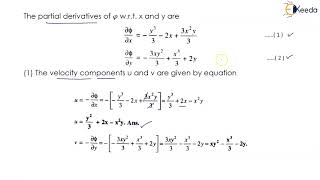
In the study of water wave motion, understanding the velocity potential is crucial. The derivation presented hinges on several core equations, primarily the Laplace equation, along with Bernoulli’s equation and the continuity equation. We begin the derivation by defining the velocity potential terms, denoted as 𝜙1, 𝜙2, 𝜙3, and 𝜙4, where dynamic boundary conditions lead us to specific expressions for each term in relation to water depth and wave dynamics.
- The governing Laplace equation is utilized alongside boundary conditions, resulting in functions of form 𝜙3 = - (𝑎𝑔/𝜎) cosh(kd) + z and 𝜙1 = - (𝑎𝑔/𝜎) cosh(kd) + z, with various dynamics affecting their signs.
- The total velocity potential is derived by summing these 𝜙 terms; this yields a result encapsulated in the formula: 𝜙 = (1/𝜎)(𝑎𝑔 cosh(kd) + z) / cosh(kd). This is crucial as it bridges dynamic wave forces and water depth.
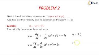
- Beyond calculating 𝜙, deriving the surface displacement (η) follows similarly, equating to a sine function of kx - σt, showcasing the periodic nature of wave phenomena.
- All calculations lead to the wave celerity equation, connecting wave speed with water depth, yielding impulsive insights into wave behavior in varying depths and illustrating the foundational principles of fluid mechanics and wave theory.
Youtube Videos

Audio Book
Dive deep into the subject with an immersive audiobook experience.
Governing Equations and Boundary Conditions
Chapter 1 of 7
🔒 Unlock Audio Chapter
Sign up and enroll to access the full audio experience
Chapter Content
I do not expect you to remember the derivation but the steps you must know the things like the specifying the governing equation, what are the governing equations governing equation is Laplace equation for the boundary conditions we utilize the Bernoulli’s equation and the continuity equation for example, so, we have obtained phi 2 here.
Detailed Explanation
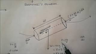
In this introduction, we focus on the governing equations necessary to derive the velocity potential. The governing equation involved here is the Laplace equation, which applies to fluid flow scenarios. Additionally, we use Bernoulli's equation to understand energy conservation in fluids and the continuity equation to ensure mass conservation. These equations provide crucial insight into how velocities and potentials are interrelated in fluid dynamics. Here, we note the derivation of phi 2, which likely represents one of the velocity potentials in our analysis.
Examples & Analogies
Consider a flowing river. The Laplace equation can be thought of as a way to describe how water runs smoothly without turbulence unless interrupted by a rock (similar to boundary conditions). Just like Bernoulli’s principle enables us to calculate how fast the water flows when it moves from a wider area to a narrower one, the governing equations help in predicting the flows of water across different scenarios.
Application of Dynamic Boundary Conditions
Chapter 2 of 7
🔒 Unlock Audio Chapter
Sign up and enroll to access the full audio experience
Chapter Content
So, if we consider phi 3 and apply the same concepts that phi 3 = you know, we apply the dynamic boundary condition. This will give C equal to D into e to the power 2 k d.
Detailed Explanation
In this part, we extend our focus to phi 3, where we apply the dynamic boundary conditions to establish the relationship between the coefficients C and D. The dynamic boundary condition accounts for fluctuating surfaces, such as water surfaces that change with wave motion. The relationship derived indicates how potentials change based on different parameters, especially when dealing with wave dynamics.
Examples & Analogies
Imagine waves crashing against a beach. The dynamic boundary condition is like observing how the waves adjust in size and speed as they encounter the shore, changing their energy state, just like how C and D behave in relation to phi 3.
Deriving Other Velocity Potentials
Chapter 3 of 7
🔒 Unlock Audio Chapter
Sign up and enroll to access the full audio experience
Chapter Content
And same procedure is repeated for the dynamic free surface boundary condition and we get for phi 3 at term like this, you understand same procedure. So phi 3 we get - ag by sigma cos h k d + z similarly, we get phi 3. And same procedure we do for phi 4, for obtaining the values.
Detailed Explanation
Here we discuss the procedure for deriving the other velocity potentials phi 3 and phi 4. By applying similar methods to the dynamic free surface boundary condition, we establish expressions that reflect the depth and wave influences on velocity potentials. Each derived potential has distinct characteristics based on the boundary conditions applied and the equations considered.
Examples & Analogies
Think of drawing water from various depths in a well. The deeper you go, the different the pressure and potential energy you analyze. Each level corresponds to a different phi, just as changes in the water level change flow characteristics and potential energies.
Summation of Velocity Potentials
Chapter 4 of 7
🔒 Unlock Audio Chapter
Sign up and enroll to access the full audio experience
Chapter Content
Now you remember I said that the total velocity potential will be the summation of the two terms. So our velocity potential is going to be phi 2 - phi 1, or also in terms of phi 3 and phi 4 also so this becomes, so if you add to velocity potential, this was you know, phi 2. And, this one with a negative sign was phi 1 so, we get this so, cos k x cos sigma t + sin k x sin sigma t can be return as cos k x - sigma t using trigonometry.
Detailed Explanation
In this segment, we summarize the findings of the previous components by stating that the total velocity potential emerges from the combination of phi 2 and phi 1, and similarly phi 3 and phi 4. The trigonometric identities help simplify the expressions, enabling us to express the total velocity potential in a clearer mathematical form. This combination essentially captures the overall behavior of wave motions under the specified conditions.
Examples & Analogies
Imagine mixing different colors of paint. Each color (phi 1, phi 2, etc.) brings its uniqueness to the final product. When you combine them, you can create a variety of shades and effects—just like adding velocity potentials yields new insights into wave behavior.
Final Formula for Velocity Potential
Chapter 5 of 7
🔒 Unlock Audio Chapter
Sign up and enroll to access the full audio experience
Chapter Content
So, the final velocity potential with the value I meanthe formula for which you are supposed to remember is this 1 ag by sigma cos h k into d + z divided by cos h k d into cos k x - sigma t this is the final velocity potential.
Detailed Explanation
This chunk provides the final expression for the velocity potential derived from previous calculations. The formula incorporates terms reflecting wave height (ag), wave angular frequency (sigma), and depth (d), along with spatial coordinates (x) and time (t). Understanding this final formula is crucial as it encapsulates the relationship between these variables and how they affect wave dynamics in a water medium.
Examples & Analogies
Consider the velocity potential as a recipe for a wave. Just like a recipe combines ingredients (wave height, depth, angles, etc.) to create a dish (the final wave), this formula encapsulates the vital components for predicting wave behavior in water.
Determining Wave Celerity
Chapter 6 of 7
🔒 Unlock Audio Chapter
Sign up and enroll to access the full audio experience
Chapter Content
So, to determine the velocity of the wave, this is the so, this is how the wave celerity that is length wave length by time period is the celerity and this is the basis of finding the way of celerity that if locate a point and traverse along the wave such that at all time t our position relative to the waveform remains fixed.
Detailed Explanation
In this section, we establish how to calculate the wave celerity, which refers to the speed at which a wave travels. This is defined as the wave's wavelength divided by the time period. By demonstrating that if we keep our position fixed relative to the wave, we can derive a relationship that simplifies the understanding of wave speed in terms of its wavelength and time period.
Examples & Analogies
Think about riding a wave on a surfboard. To stay on top of the wave as it moves towards the shore, you must paddle at a speed that matches the wave’s speed—this is akin to matching the wave's celerity and keeping your position relative to the wave constant.
Dispersion Relationship
Chapter 7 of 7
🔒 Unlock Audio Chapter
Sign up and enroll to access the full audio experience
Chapter Content
Now, one important thing after this derivation of the velocity potential is something called a dispersion relationship that is one of the core concept of the wave mechanics.
Detailed Explanation
This final chunk discusses the concept of dispersion relationships, a fundamental aspect of wave mechanics that relates wave speed to wavelength, period, and water depth. It highlights how different conditions affect wave motion and the way waves propagate through a medium, establishing a crucial understanding of fluid dynamics in wave analyses.
Examples & Analogies
Think about how different sounds travel in air depending on their frequency. A bass note travels slower than a treble note. Similarly, in water, waves of different wavelengths travel at different speeds, illustrating the importance of dispersion relationships in wave mechanics.
Key Concepts
-
Laplace equation: A central equation for determining the velocity potential.
-
Boundary conditions: Conditions that govern how wave potentials are defined at surfaces.
-
Velocity potential formula: The derived expression encapsulating wave motion dynamics.
Examples & Applications
If a wave travels in water of depth d, the velocity potential can be derived using predefined constants and conditions.
An example relationship where if a wave period T is known, one can calculate wave celerity using C = L/T.
Memory Aids
Interactive tools to help you remember key concepts
Rhymes
When waves do sway and dance in air,
Stories
Once upon a time, waves danced across the ocean. They whispered secrets of their speed to anyone who listened, teaching sailors to navigate by understanding their depth and time taken, weaving the magical formula, C=L/T.
Memory Tools
Remember the acronym WAVE: Wavelength, Amplitude, Velocity, Energy - fundamentals for wave mechanics.
Acronyms
Use the acronym BCD for Boundary Conditions and Dynamics, key to understanding wave behavior.
Flash Cards
Glossary
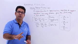
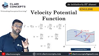
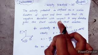
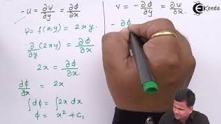
- Velocity Potential (𝜙)
A scalar function whose gradient gives the velocity field in fluid mechanics.
- Laplace Equation
A second-order partial differential equation fundamental in potential theory.
- Bernoulli’s Equation
An equation describing the conservation of energy in a fluid flow.
- Celerity (C)
The speed of wave propagation in the medium, often expressed as L/T.
- Dispersion Relationship
A relationship that describes how wave speed depends on wavelength and depth.
Reference links
Supplementary resources to enhance your learning experience.