
Introduction
Enroll to start learning
You’ve not yet enrolled in this course. Please enroll for free to listen to audio lessons, classroom podcasts and take practice test.
Interactive Audio Lesson
Listen to a student-teacher conversation explaining the topic in a relatable way.
Understanding Normal Distribution
🔒 Unlock Audio Lesson
Sign up and enroll to listen to this audio lesson

Today, we're diving into the Normal Distribution. It's often referred to as the Gaussian distribution. Can anyone tell me why it's called 'normal'?

I think because it's common in nature, right?
Exactly! The Normal Distribution appears in many real-world situations. It's key to understanding randomness. Now, can anyone explain what defines a Normal Distribution?

Is it defined by the mean and standard deviation?
Yes! That's correct. The mean (μ) is the center, and the standard deviation (σ) measures how spread out the data is. It creates that bell-shaped curve we often see in graphs.

What makes the shape so important?
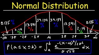
Good question! The symmetry and the properties around the mean tell us a lot about the data distribution. For example, according to the Empirical Rule, 68% of data falls within ±1σ.

So, if we know the mean and standard deviation, we can predict where most data points will fall?
Exactly! Now, can you all summarize the importance of the Normal Distribution?
It's fundamental in statistics and helps describe a wide range of phenomena!
Exploring Properties
🔒 Unlock Audio Lesson
Sign up and enroll to listen to this audio lesson

Let’s explore some properties in more detail. Who can remind us how the Normal Distribution is shaped?
It's bell-shaped and symmetrical!
Right! And what does this symmetry tell us about the mean, median, and mode?
They’re all equal in a Normal Distribution.
Correct! One more important property: the total area under the curve equals what?
One! It represents the total probability.
Exactly! This area is crucial for calculating probabilities. Now, who remembers the Empirical Rule?
Oh! It says that about 68% of values lie within one standard deviation from the mean!
Fantastic! And what about two and three standard deviations?
Around 95% and 99.7%!
Great summary! The Empirical Rule helps visualize how data is spread.
Applications of Normal Distribution
🔒 Unlock Audio Lesson
Sign up and enroll to listen to this audio lesson
Now, let's discuss where we can see the Normal Distribution in real life. Can someone give an example?
I think test scores often follow a Normal Distribution?
Yes! Other examples include heights and measurement errors. However, what’s a limitation of the Normal Distribution?
When data is heavily skewed or has extreme values.
Exactly! While it's a powerful tool, we must check the data's symmetry. Can you think of cases where transformation might be necessary?
Like converting skewed data using logarithm transformation?
Yes! By applying transformations, we can apply the principles of Normal Distribution more effectively.
Introduction & Overview
Read summaries of the section's main ideas at different levels of detail.
Quick Overview
Youtube Videos

Audio Book
Dive deep into the subject with an immersive audiobook experience.
Overview of Normal Distribution
Chapter 1 of 1
🔒 Unlock Audio Chapter
Sign up and enroll to access the full audio experience
Chapter Content
The Normal Distribution, also called the Gaussian distribution, is a continuous probability distribution fundamental in statistics and probability. It describes many real-world random phenomena—like heights, test scores, measurement errors—and is key due to the Central Limit Theorem, which tells us that sums of many independent random variables tend to be normally distributed.
Detailed Explanation
The Normal Distribution, or Gaussian distribution, is essential in statistics and is used to model a variety of real-world situations. These can include things like the distribution of people's heights or test scores. One of the critical reasons it's so useful in statistics is due to the Central Limit Theorem, which states that when you add together many independent random variables, the result will tend to follow a Normal distribution, regardless of the original distribution of those variables. This makes it a cornerstone of statistical analysis.
Examples & Analogies
Imagine a huge jar where 40% of the marbles are red. You repeatedly take handfuls of 50 marbles each (independent samples). For every handful, you record the proportion of red marbles \(\hat p\).
- If you collect many such proportions, their histogram will look bell-shaped (Normal).
- The distribution of \(\hat p\) is approximately:
\[
\hat p \approx \text{Normal}\!\left(0.40,\; \sqrt{\frac{0.4 \cdot 0.6}{50}}\right)
= \text{Normal}(0.40,\; 0.0693)
\]
Key Concepts
-
Normal Distribution: A fundamental continuous probability distribution characterized by its mean and standard deviation.
-
Bell-shaped Curve: Visual representation of the Normal Distribution, symmetrical around the mean.
-
Empirical Rule: A statistical guideline regarding how data is distributed in relation to the mean and standard deviation.
-
Standard Normal Distribution: A special case of Normal Distribution where the mean is 0 and the standard deviation is 1.
-
Central Limit Theorem: States that the sum of a large number of independent random variables will be normally distributed.
Examples & Applications
Test scores in a large class are often normally distributed; understanding their distribution helps in evaluating student performance.
Heights of individuals in a population typically align with a Normal Distribution pattern, allowing for predictions about height ranges.
Memory Aids
Interactive tools to help you remember key concepts
Rhymes
To understand the normal shape each time, remember bell and symmetry combined.
Stories
Once upon a time in Statland, all the heights of the people fell in a perfect bell shape, balanced around the average. The people who were taller or shorter were fewer, creating a wonderful community of symmetry!
Memory Tools
For the Empirical Rule, remember 68, 95, 99.7 - just think of a race where runners take their spots centered at the mean.
Acronyms
Use the acronym 'SPE' for 'Symmetric, Parameters (Mean & SD), Empirical Rule' to remember the key features of Normal Distribution.
Flash Cards
Glossary
- Normal Distribution
A continuous probability distribution characterized by its bell shape and defined by its mean (μ) and standard deviation (σ).
- Mean (μ)
The average value of a set of numbers, which is the center point of the Normal Distribution.
- Standard Deviation (σ)
A measure of the amount of variation or dispersion of a set of values.
- Empirical Rule
A statistical rule stating that for a Normal Distribution, approximately 68% of the data falls within one standard deviation, 95% within two, and 99.7% within three standard deviations from the mean.
- Central Limit Theorem
The theorem stating that the sum of a large number of independent random variables will approach a Normal Distribution.
Reference links
Supplementary resources to enhance your learning experience.