
Probability Distributions (Discrete)
Enroll to start learning
You’ve not yet enrolled in this course. Please enroll for free to listen to audio lessons, classroom podcasts and take practice test.
Interactive Audio Lesson
Listen to a student-teacher conversation explaining the topic in a relatable way.
Introduction to Discrete Probability Distributions
🔒 Unlock Audio Lesson
Sign up and enroll to listen to this audio lesson

Today, we’re diving into discrete probability distributions. Can anyone tell me what a probability distribution is?

I think it’s about how we represent outcomes and their likelihood?
Exactly! A probability distribution assigns probabilities to specific outcomes. Can anyone tell me what conditions must be met for these probabilities?

They must add up to one and each probability has to be between zero and one.
Great! To remember this, think '0 to 1, sum it is done!'

That’s a fun way to remember it!
Let's summarize: probabilities must be non-negative and sum to one. Now, who can tell me what the expected value is?

Isn't it the average of all possible values?
Correct! The expected value gives us a measure of the center of a probability distribution.
Calculating Expected Value and Variance
🔒 Unlock Audio Lesson
Sign up and enroll to listen to this audio lesson

Now that we know what expected value is, let’s see how we actually calculate it. Can anyone provide the formula?
I think it’s E(X) = sum of xᵢ * pᵢ?
Exactly, wonderful! What about variance? How do we find that?
It's the sum of the squares of differences from the expected value?
Right! Variance tells us how spread out the probabilities are. Formula for that is Var(X) = sum of (xᵢ - E(X))² * pᵢ.
Can you give us a practical example?
Of course! Let’s roll a fair die. What’s the expected value?
It should be 3.5.
Correct! And we'll calculate variance next.
Application of Discrete Probability Distributions
🔒 Unlock Audio Lesson
Sign up and enroll to listen to this audio lesson
Let’s talk about how discrete probability distributions are used in real life. Can anyone think of an example?
Lottery games, where each number has a different probability.
Good example! In lotteries, each outcome is discrete and has an associated probability. What about another real-world application?
When tossing a coin, we can predict heads or tails probabilities.
Absolutely! This kind of probability analysis is crucial in risk assessments. It lets us gauge uncertainty in various situations.
Do we always have to use complex calculations for these probabilities?
Not always. Sometimes we can estimate them based on past data—this is where empirical probability comes into play.
That makes sense!
Common Mistakes and Review
🔒 Unlock Audio Lesson
Sign up and enroll to listen to this audio lesson
As we wrap up our discussion today, what are some common mistakes we could avoid in dealing with probability distributions?
Confusing independent vs. mutually exclusive events?
Exactly! That’s a big one. Can someone provide a quick definition of those terms?
Independent events don’t affect each other; mutually exclusive events cannot happen at the same time.
Well said! Remember those definitions. Lastly, let’s recap—who can summarize what we learned?
We covered discrete probability distributions, expected values, variances, and real-life applications.
Fantastic summary! Always ensure when assigning probabilities, they meet the key conditions. Great work today!
Introduction & Overview
Read summaries of the section's main ideas at different levels of detail.
Quick Overview
Standard
In this section, we explore discrete probability distributions where outcomes have associated probabilities. Key concepts include the properties of probabilities, expected value, and variance. The section also highlights the need for probabilities to sum to one, along with an example of a fair die roll to illustrate expected value and variance.
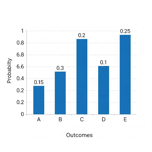
Probability Distribution bar chart sample:
Detailed
Probability Distributions (Discrete)
In probability theory, discrete probability distributions provide a way to characterize random variables that can take on specific discrete values. Each outcome, denoted as X, has a corresponding probability assigned to it, resulting in a series of outcomes and probabilities: p₁, p₂, ..., pₙ. For a valid probability distribution:
- The sum of all probabilities must equal one: ∑pᵢ = 1.
- Each individual probability must lie between zero and one: 0 ≤ pᵢ ≤ 1.
Key Definitions
- Expected Value (Mean): The expected value (E(X)) of a discrete random variable gives a measure of the central tendency of the random variable. It is calculated as:
E(X) = ∑(xᵢ * pᵢ)
- Variance: Variance (Var(X)) measures how much the values of the random variable differ from the expected value. It is given by:
Var(X) = ∑((xᵢ - E(X))² * pᵢ)
Example
Rolling a fair die:
- The expected value of rolling a die can be calculated as:
E(X) = (1/6)1 + (1/6)2 + (1/6)3 + (1/6)4 + (1/6)5 + (1/6)6 = 3.5
- The variance can be calculated similarly, leading to a more detailed understanding of the distribution of outcomes. By grasping these concepts, students can understand how probabilities apply to various discrete scenarios.
Audio Book
Dive deep into the subject with an immersive audiobook experience.
Discrete Random Variables and Their Probabilities
Chapter 1 of 5
🔒 Unlock Audio Chapter
Sign up and enroll to access the full audio experience
Chapter Content
• Outcome X takes values x₁, x₂, … xₙ with probabilities p₁, p₂, … pₙ.
Detailed Explanation
In this context, a discrete random variable X is one that can take on a finite or countably infinite number of separate values. For example, when you roll a die, the outcome (let's say X) can be 1, 2, 3, 4, 5, or 6. Each of these outcomes corresponds to a probability, denoted p₁, p₂, ..., and so on, where p represents the chance of each value occurring.
Examples & Analogies
Think of a jar filled with colored marbles. If you take one marble out at random, the possible outcomes are the colors of the marbles present (like red, blue, green, etc.), and each color has a specific chance of being picked based on the total number of marbles.
Probability Requirements
Chapter 2 of 5
🔒 Unlock Audio Chapter
Sign up and enroll to access the full audio experience
Chapter Content
• Must satisfy: ∑pᵢ = 1 and 0 ≤ pᵢ ≤ 1.
Detailed Explanation
The probabilities associated with the outcomes of a discrete random variable must meet two crucial conditions: the sum of the probabilities of all possible outcomes must equal 1. This means that when you consider all possible events, something must happen. Additionally, each individual probability must be between 0 and 1, meaning it can't be less than impossible (0) or more than certain (1).
Examples & Analogies
If we return to our marble jar, if we know there are 10 marbles total, and 3 are red, then the probability of pulling a red marble is 3/10 (which is 0.3). If you sum the probabilities of all colors (like red, blue, green), they should add up to 1, meaning there's a complete certainty that you will pull one color, no matter which one it is.
Expected Value (Mean)
Chapter 3 of 5
🔒 Unlock Audio Chapter
Sign up and enroll to access the full audio experience
Chapter Content
• Expected value (mean): 𝐸(𝑋) = ∑𝑥 𝑝 .
Detailed Explanation
The expected value, or mean, of a discrete random variable X is calculated by multiplying each possible outcome by its probability and then summing all these products. This measure provides a single value that represents the average or 'center' of the distribution of outcomes—basically, it is what you would expect to happen on average over many trials.
Examples & Analogies
Imagine you're playing a game where if you roll a die you earn a number of points equal to the number rolled. If you calculate the expected number of points you will earn from rolling the die repeatedly, you'd take each outcome (1 through 6), multiply by its probability (1/6), and find that the expected value is 3.5 points.
Variance of a Discrete Random Variable
Chapter 4 of 5
🔒 Unlock Audio Chapter
Sign up and enroll to access the full audio experience
Chapter Content
• Variance: 𝑉𝑎𝑟(𝑋) = ∑(𝑥 −𝐸(𝑋)) 𝑝 .
Detailed Explanation
Variance measures the spread or dispersion of a set of outcomes of a random variable. It is the average of the squared differences from the expected value. A high variance indicates that the outcomes are spread out widely around the mean, while a low variance indicates that they are clustered closely around the mean.
Examples & Analogies
Continuing with our die-rolling game, if the variance in the points earned is low, this means your scores when rolling the die won't fluctuate much—you might consistently score around 3.5 points. However, if the variance is high, some rolls could yield very low or very high scores, making the game unpredictable.
Example: Rolling a Fair Die
Chapter 5 of 5
🔒 Unlock Audio Chapter
Sign up and enroll to access the full audio experience
Chapter Content
• Example: Rolling a fair die → E(X)=3.5, Var(X)=35/12.
Detailed Explanation
In the example of rolling a fair die, we can calculate both the expected value and variance. The expected value E(X) is calculated based on the outcomes {1, 2, 3, 4, 5, 6} and their equal probabilities (1/6). This gives us an average outcome of 3.5. The variance can be computed similarly using the formula provided, leading to a numerical value representing how far the outcomes typically deviate from the mean.
Examples & Analogies
Imagine a group of friends playing a board game that uses a fair die. If they record their scores from multiple rounds, they’ll find that over many games, their average score tends to even out to 3.5, and some scores occasionally float far above or below this average, as reflected in the variance of their rolls.
Key Concepts
-
Discrete Probability Distribution: This reflects the probabilities of individual outcomes for discrete random variables.
-
Expected Value: A critical measurement used to denote the average outcome, derived from possible values weighted by their likelihood.
-
Variance: Provides insight into the variability of a probability distribution relative to its expected value.
Examples & Applications
Example: Rolling a fair die where the probabilities for each side are equal, leading to an expected value of 3.5.
Example: A biased coin toss scenario, showcasing how different probabilities can affect expected outcomes.
Memory Aids
Interactive tools to help you remember key concepts
Rhymes
Sum it up, make it one, from zero to one—find your fun!
Stories
Imagine rolling dice in a game where luck decides the average score and probability becomes your guide.
Memory Tools
E for Expected, V for Variance—EVV: Evaluate Variance for Value.
Acronyms
SPICE
Sum of Probabilities Increases; Check Expected values!
Flash Cards
Glossary
- Discrete Probability Distribution
A distribution that shows the probabilities of outcomes for a discrete random variable.
- Expected Value
The average or mean value of a random variable; a measure of center.
- Variance
A measure of the dispersion of a set of probabilities around the expected value.
Reference links
Supplementary resources to enhance your learning experience.