
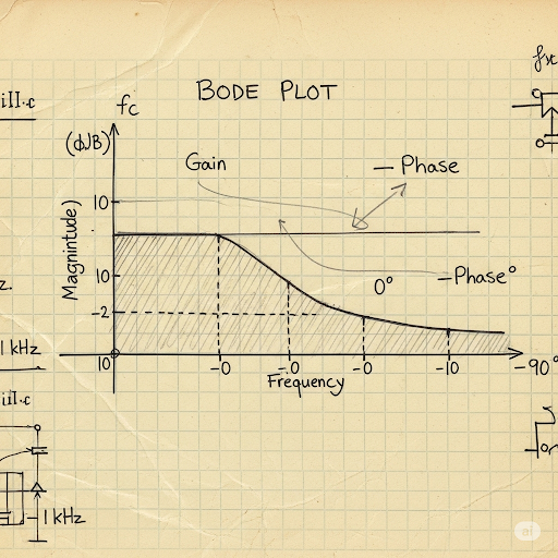
Bode Plot Sketch
Enroll to start learning
You’ve not yet enrolled in this course. Please enroll for free to listen to audio lessons, classroom podcasts and take practice test.
Interactive Audio Lesson
Listen to a student-teacher conversation explaining the topic in a relatable way.
Understanding Gain Expressions
🔒 Unlock Audio Lesson
Sign up and enroll to listen to this audio lesson

Let's start by discussing how the gain expression changes with frequency. Can anyone tell me what the denominator of the gain expression looks like?

I think it includes terms like '1 + gR', right?
Exactly! And what about for higher frequencies?

That would mean that the 'sRC' term becomes significant.
Correct! This leads to a pole and a zero in our analysis. Can someone explain what they understand by poles and zeros?

Poles are points where gain drops, and zeros are where the gain is maximized.
Great! Remembering that poles lower the response while zeros boost it is crucial.
To summarize, we restructured the gain expression to reveal how frequency affects the output.
Identifying Poles and Zeros
🔒 Unlock Audio Lesson
Sign up and enroll to listen to this audio lesson

Let's analyze the impact of our poles and zeros further. How do we determine their positions in the Bode plot?

I guess we derive them from the gain expression we discussed earlier?
Yes! And what happens to the gain magnitude as it reaches these critical points?
At the zero, the gain increases significantly, right?
Correct! And beyond the pole, what occurs?
The gain starts to drop.
Exactly! Always note that zeros increase gain while poles bring it down. That's fundamental for sketching Bode plots.
To recap: we've established how to identify poles and zeros for an amplifier's frequency response.
Frequency Response Characteristics
🔒 Unlock Audio Lesson
Sign up and enroll to listen to this audio lesson
Now let’s look at how the self-bias configuration influences our frequency response. Can anyone highlight how it differs from fixed bias?
The self-bias configuration leads to lower cutoff frequencies before the effect of capacitors kicks in.
Good observation! What happens once we exceed our corner frequency?
The response levels out, approaching that of the fixed bias configuration.
Exactly. We transition from one behavior to another as frequency increases. Can you visualize this transition in our Bode plot?
Yes! Initially, it starts at a certain gain, then rises, and eventually levels out.
Well done! Summarizing this session, the bias configuration significantly shapes our frequency response and gain behavior.
Real-World Implications
🔒 Unlock Audio Lesson
Sign up and enroll to listen to this audio lesson
Finally, we need to understand the practical implications of what we've learned. How does this knowledge influence our circuit design?
It helps in selecting components with appropriate cutoff frequencies.
Exactly! What would happen if our cutoff frequency is too low?
We risk losing important frequency components of the signal.
Precisely! Therefore, engineers need to balance component values carefully. Can you recall what we discussed about capacitor values?
Capacitors should be sized sufficiently to ensure a broad bandwidth.
Great summary! In this session, we connected theory to practical aspects that are essential for effective amplifier design.
Introduction & Overview
Read summaries of the section's main ideas at different levels of detail.
Quick Overview
Standard
The focus of this section is on understanding the Bode plot for Common Emitter (CE) amplifiers with specific attention to frequency response, gain expressions, and crucial points where poles and zeros affect behavior. It illustrates how the gain varies with frequency and outlines how to differentiate between fixed bias and self-bias configurations.
Detailed
Bode Plot Sketch in CE Amplifiers
This section provides an analytical framework for sketching the Bode plot of Common Emitter (CE) amplifiers, particularly those employing self-bias configurations with capacitors. We begin by addressing the impact of capacitors on the frequency response of the amplifier, leading to the identification of zeros and poles in the gain function. Through expressions derived from circuit analysis, the key elements being evaluated include:
- Gain Expression Restructuring: The narrator explains how the gain from input to output is restructured to isolate frequency-dependent terms.
- Frequency Response Characteristics: The way that the frequency response is affected by the presence of capacitors results in defining critical points (poles and zeros).
- Practical Implications on Gain: It clarifies that the gain at low frequencies mirrors that of a self-biased circuit without capacitors until a certain corner frequency is reached, after which the gain stabilizes to match that of a fixed bias configuration.
- Incorporation of Additional Components: The role of coupling capacitors is also mentioned, including high-pass and low-pass behaviors that affect the overall output characteristics.
- Numerical Examples and Cutoff Frequencies: Concrete examples illustrate the calculation of critical frequencies (lower and upper cutoff) and insight into practical implications for amplifier design.
This section is pivotal as it lays the groundwork for understanding the response of CE amplifiers across different frequency regimes, thereby informing practical circuit design rooted in theoretical analysis.
Youtube Videos

Audio Book
Dive deep into the subject with an immersive audiobook experience.
Understanding Bode Plots
Chapter 1 of 5
🔒 Unlock Audio Chapter
Sign up and enroll to access the full audio experience
Chapter Content
So, let me clear and then let me try to plot the gain or magnitude plot of this A. So, A is having; of course, we do have low frequency gain something like this and which is assuming that this part it is more than 1. So, we can see that it is above 0 dB. So, it is having a gain like this. So, which is coming from this part and then we do have one 0 here.
Detailed Explanation
In this chunk, we are discussing how to sketch a Bode plot for a given gain function. The Bode plot is a graphical representation of a linear, time-invariant system transfer function. Here, we focus on the low-frequency gain, which is depicted as a magnitude plot above 0 dB, indicating that the gain at lower frequencies is greater than one (1). The presence of a zero on the plot signifies a frequency at which the gain starts to rise significantly, making the overall shape of the plot critical for understanding the amplifier's frequency response.
Examples & Analogies
Think of a Bode plot as a speedometer for an amplifier, showing how it responds differently at various frequencies, much like how a car responds differently at varying speeds on the road. Just as a driver needs to know how fast a car can go at different gears, engineers need to understand how amplifiers behave at different frequencies.
Pole and Zero Behavior
Chapter 2 of 5
🔒 Unlock Audio Chapter
Sign up and enroll to access the full audio experience
Chapter Content
Now, this is independent of frequency, this is also independent of frequency; we can take together. So, 1 + g R you can take them together. And then if you take this factor as out, we do have 1 +. So, what we have here it is; one part is this one, which is independent of s, independent of the frequency and then we do have the other part, it is dependent on frequency.
Detailed Explanation
This section highlights how we can simplify the gain function by isolating frequency-independent and frequency-dependent components. We discuss a combination where some terms do not change with frequency (like 1 + gR) while others are frequency-dependent. The critical observation here is that, by separating these components, we can more easily analyze how the amplifier's gain varies with frequency. This reflects the overall Bode plot's shape and aids in identifying key characteristics such as poles and zeros.
Examples & Analogies
Imagine mixing paint colors. Some colors are permanent and won’t change regardless of the medium you use (the frequency-independent components). In contrast, other colors may shift or change intensity when diluted or altered with different supplies (the frequency-dependent components). This analogy helps in understanding how different factors affect the overall output in a system.
Impact of Poles and Zeros
Chapter 3 of 5
🔒 Unlock Audio Chapter
Sign up and enroll to access the full audio experience
Chapter Content
In fact, if you recall that, this part it is same as the previous case when the C was not there. And due to the C, then we do have this additional part and note that it is having a zero at s = 0 and also a pole at s = -R.
Detailed Explanation
The chunk discusses how adding a capacitor (C) influences the system’s response. When this capacitor is introduced, new dynamics take effect, resulting in a zero and a pole presented on the Bode plot. A zero at s = 0 indicates a frequency point where the gain boosts, while a pole signifies where the gain will drop off at high frequencies. Understanding the impact of each pole and zero is crucial to effectively use amplifiers in different applications.
Examples & Analogies
Consider tuning a radio. When you adjust the dial (frequency), you might suddenly hear a station clearly at one moment (the zero), but if you keep adjusting you can also find spots where the sound fades away or becomes distorted (the poles). Just like the radio's response changes with each frequency, the amplifier responds uniquely at different points due to its poles and zeros.
Cutoff Frequencies
Chapter 4 of 5
🔒 Unlock Audio Chapter
Sign up and enroll to access the full audio experience
Chapter Content
Now, depending on the value of this C of course, it is possible that this corner frequency it may exceed this corner frequency. But most of the time what we do, we take the value of this C sufficiently high, so that this corner frequency it is not exceeding this one.
Detailed Explanation
In this section, we emphasize the importance of choosing the capacitor size (C) when determining the cutoff frequency. A larger value of C is typically chosen to ensure the cutoff frequency remains within acceptable limits for the application. If C is too small, it could result in an undesired shift in the cutoff frequency, which could adversely affect the amplifier's performance in its intended frequency range.
Examples & Analogies
Think about a water filtration system. If the filter (analogous to C) is too small, it won’t be able to handle the needs of a big household (the frequency range), leading to poor performance. However, if it's appropriately sized, it will effectively filter out unwanted elements, ensuring clean water (clear sound) is delivered consistently.
Determining the Lower Cutoff Frequency
Chapter 5 of 5
🔒 Unlock Audio Chapter
Sign up and enroll to access the full audio experience
Chapter Content
So, what we are saying is that, let me write in terms of ω, lower cutoff frequency if I say ω = max of these two candidates; one is dependent on R and C, the other on R.
Detailed Explanation
This chunk explains the method for determining the lower cutoff frequency of the circuit based on two candidates derived from the capacitor and resistor values. By taking the maximum value of these candidates, the accurate lower cutoff frequency can be discerned. This ensures that the amplifier operates effectively above this cutoff point, allowing the expected performance across the desired frequency range.
Examples & Analogies
Imagine setting a speed limit for a race. You want to ensure that cars can’t go below a certain speed to keep up with the race dynamics (the lower cutoff frequency). So, you choose the highest of two proposed speed limits to ensure safety and optimal speed throughout the race, just as engineers do when selecting cutoff frequencies.
Key Concepts
-
Gain Expression: The gain from input to output in a CE amplifier depends on frequency conditions.
-
Poles and Zeros: Key points in the response that significantly influence the gain characteristics.
-
Frequency Response: Understanding how an amplifier reacts at various frequencies is crucial for effective design.
Examples & Applications
If a CE amplifier shows a gain of 20 dB at low frequencies, this might change at the corner frequency where a pole appears, dropping the gain.
In a scenario where the capacitor's value is increased significantly, the frequency response of the amplifier shifts, affecting both the zero and pole locations.
Memory Aids
Interactive tools to help you remember key concepts
Rhymes
Poles bring down the gain, while zeros give it gain! Remember this once and again!
Stories
Imagine an amplifier in a race. As it approaches zero, it speeds up and gains elevation. But when it reaches a pole, its speed decreases until it levels off.
Memory Tools
Zero = Zoom up (gain increase), Pole = Plunge down (gain decrease).
Acronyms
GPP
Gain
Poles
Poles—understand how each influences frequency response!
Flash Cards
Glossary
- Bode Plot
A graph of the frequency response of a system that displays magnitude (gain) and phase of a signal against frequency.
- Gain
The ratio of output voltage to input voltage in a circuit, often expressed in decibels (dB).
- Poles
Frequency points where the gain of a system drops to zero; these points indicate a decrease in output.
- Zeros
Frequency points where the gain of a system increases significantly; these points indicate an increase in output.
- Frequency Response
The measure of a circuit's output spectrum in response to an input signal and describes how the circuit responds at different frequencies.
Reference links
Supplementary resources to enhance your learning experience.