
Gradient Descent Variants
Enroll to start learning
You’ve not yet enrolled in this course. Please enroll for free to listen to audio lessons, classroom podcasts and take practice test.
Interactive Audio Lesson
Listen to a student-teacher conversation explaining the topic in a relatable way.
Batch Gradient Descent
🔒 Unlock Audio Lesson
Sign up and enroll to listen to this audio lesson

Today, we're discussing Batch Gradient Descent. Can anyone describe what it is?

Isn't it when you use all the training examples to compute the gradient?
Exactly! This means we calculate the average gradient of the complete dataset before updating the weights. It’s stable but can be slow with large datasets. A good memory aid is thinking of it like baking a batch of cookies, where you make them all at once.

What are the drawbacks?
Good question! The main drawback is computational time, especially with big data. So what could be an alternative?

Maybe Stochastic Gradient Descent?
That's correct! Let’s explore that next.
Stochastic Gradient Descent
🔒 Unlock Audio Lesson
Sign up and enroll to listen to this audio lesson

Now, let’s dive into Stochastic Gradient Descent, or SGD. How is it different from Batch Gradient Descent?

It updates the weights after each training sample instead of waiting for the entire dataset!
Exactly! This can lead to faster convergence, but the path to convergence tends to be noisy. It’s like sprinting; you make quick progress but can be erratic. Can anyone think of the pros and cons?
The pro is speed, but the con is potential instability.
That's right! Now, what do you think a practical solution to the instability could be?
Maybe combining the two approaches?
Spot on! That brings us to Mini-batch Gradient Descent.
Mini-batch Gradient Descent
🔒 Unlock Audio Lesson
Sign up and enroll to listen to this audio lesson
Mini-batch Gradient Descent combines Batch and SGD. Why do you think this method might be advantageous?
It balances the stability of Batch with the speed of SGD.
Exactly! It divides the training dataset into small batches, providing a reliable update frequency while speeding up computations. A good analogy here is packing meals into small containers rather than taking the whole kitchen.
That definitely makes sense! What about the learning rate adjustments?
Great follow-up! With Mini-batch, we can also implement adaptive learning rate strategies. Let’s explore some popular optimizers next.
Optimizers (Adam, RMSProp, Adagrad)
🔒 Unlock Audio Lesson
Sign up and enroll to listen to this audio lesson
Now, let’s discuss some advanced optimizers. Who's familiar with Adam?
Is it like an enhancement to gradient descent?
Right! Adam combines the benefits of AdaGrad and RMSProp. It adapts the learning rate based on first and second moments of gradients. Why might that be beneficial?
It helps in dealing with sparse gradients!
Exactly! What about RMSProp?
It adjusts the learning rate based on the average gradient, right?
Yes! And finally, Adagrad adapts the learning rate for each parameter. Why is that useful?
It helps deal with parameters that have infrequent updates!
That’s correct! Each optimizer has its strengths and works best under different circumstances. Excellent discussion today!
Introduction & Overview
Read summaries of the section's main ideas at different levels of detail.
Quick Overview
Standard
In this section, we explore various gradient descent variants such as Batch, Stochastic, and Mini-batch Gradient Descent. Additionally, we examine popular optimizers like Adam, RMSProp, and Adagrad that enhance the performance of the gradient descent algorithm.
Detailed
Gradient Descent Variants
Gradient descent is a cornerstone technique in training deep neural networks. It minimizes the loss function to improve model accuracy. This section discusses the three main variants:
- Batch Gradient Descent: Processes the entire training dataset in one step to compute the average gradient. This method is stable but can be slow with large datasets.
- Memory Aid: Think of it as a batch of cookies—baking all at once versus one at a time.
- Stochastic Gradient Descent (SGD): Updates weights using each training example individually, introducing more noise to the training process but often achieving faster convergence.
- Memory Aid: Imagine running a race where you sprint forward at each step without waiting.
- Mini-batch Gradient Descent: A compromise between Batch and SGD; it divides the dataset into small batches. This approach benefits from both methods by balancing speed and variance.
- Memory Aid: Consider packing meals into small containers instead of taking the whole kitchen.
Additionally, we discuss advanced optimizers like:
- Adam: Combines the advantages of two other extensions—AdaGrad and RMSProp.
- RMSProp: Adjusts the learning rate based on average gradients.
- Adagrad: Adaptively scales the learning rate for each parameter.
These variants and optimizers are crucial for effectively training deep learning models, ensuring scalability and efficiency.
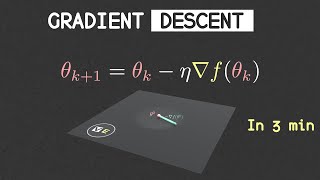
Youtube Videos
Audio Book
Dive deep into the subject with an immersive audiobook experience.
Batch Gradient Descent
Chapter 1 of 4
🔒 Unlock Audio Chapter
Sign up and enroll to access the full audio experience
Chapter Content
• Batch Gradient Descent
Detailed Explanation
Batch Gradient Descent involves calculating the gradient of the loss function using the entire dataset. This means that for every update of the model parameters, the algorithm waits until it has seen all training examples.
This approach typically leads to a stable and smooth convergence path but can be computationally expensive, especially with large datasets.
Examples & Analogies
Think of Batch Gradient Descent like trying to gauge how well a restaurant is doing by waiting for all the customers to finish their meals before making any decisions on the menu or service improvements. You get a clear overall picture, but it takes time to gather all the data.
Stochastic Gradient Descent (SGD)
Chapter 2 of 4
🔒 Unlock Audio Chapter
Sign up and enroll to access the full audio experience
Chapter Content
• Stochastic Gradient Descent (SGD)
Detailed Explanation
Stochastic Gradient Descent, on the other hand, updates the model parameters using only one training example at a time. This can lead to faster updates and can help the algorithm to escape local minima, resulting in potentially better solutions. However, the error can fluctuate significantly, leading to a noisier convergence path.
Examples & Analogies
Imagine Stochastic Gradient Descent as a person trying to make a recipe by adding one ingredient at a time, taste-testing each time before moving on. This method allows for quick adjustments but can also lead to inconsistent flavor outcomes if one tastes too frequently.
Mini-batch Gradient Descent
Chapter 3 of 4
🔒 Unlock Audio Chapter
Sign up and enroll to access the full audio experience
Chapter Content
• Mini-batch Gradient Descent
Detailed Explanation
Mini-batch Gradient Descent is a middle ground between Batch and Stochastic Gradient Descent. In this approach, the algorithm splits the dataset into small batches and then calculates the gradient for each batch. This method benefits from the stability of batch learning while retaining the speed advantages of stochastic learning.
Examples & Analogies
Mini-batch Gradient Descent is like a teacher who gives quizzes to small groups of students instead of the entire class at once. This allows for quicker feedback for each group (like smaller batches) while still providing a comprehensive understanding of the material overall.
Optimizers Overview
Chapter 4 of 4
🔒 Unlock Audio Chapter
Sign up and enroll to access the full audio experience
Chapter Content
• Optimizers:
o Adam
o RMSProp
o Adagrad
Detailed Explanation
Optimizers are advanced algorithms that adjust the learning rate itself dynamically to improve convergence speed. For instance:
- Adam adjusts the learning rate based on the average of recent gradients, making it efficient and effective.
- RMSProp adapts the learning rate for each parameter based on the recent gradients, which helps in stabilizing the training process.
- Adagrad modifies the learning rate based on the parameters' historical gradients, allowing larger updates for infrequent parameters and smaller updates for frequent parameters.
Examples & Analogies
Think of these optimizers like personal trainers who adjust your workout intensity based on your progress. Adam provides personalized adjustments based on your recent results, RMSProp tailors exercises according to your performance in specific activities, and Adagrad modifies the plan based on how often you do certain exercises.
Key Concepts
-
Batch Gradient Descent: Updates model weights using the entire dataset to compute gradients, leading to stable updates.
-
Stochastic Gradient Descent (SGD): Updates model weights using individual training examples, resulting in faster but noisier convergence.
-
Mini-batch Gradient Descent: Utilizes small batches for weight updates, combining the benefits of stability and speed.
-
Adam Optimizer: An algorithm that adjusts learning rates based on momentum and helps improve convergence in neural networks.
-
RMSProp: An optimizer that modifies the learning rate dynamically based on recent gradients, aiding in faster convergence.
-
Adagrad: An optimizer that enables adaptive learning rates for each parameter, enhancing performance in sparse data scenarios.
Examples & Applications
In practice, Batch Gradient Descent is often used for smaller datasets to ensure stable convergence, while Stochastic Gradient Descent can be applied to live data or larger datasets for quicker updates.
Mini-batch Gradient Descent is commonly used in modern deep learning frameworks like TensorFlow and PyTorch to balance computation efficiency with model accuracy.
For instance, Adam is widely used in training deep learning models due to its efficient computation and adaptability with complex datasets.
Memory Aids
Interactive tools to help you remember key concepts
Rhymes
Batch by the batch, we gather the data, while Stochastic runs fast, like the heart of a skater.
Stories
Once upon a time in DataLand, the wise Batch always took his time while Stochastic would rush to the finish line. Mini-batch found the perfect path, combining speed and grace to achieve great math.
Memory Tools
B-S-M or 'Big Steps Matter': Remember Batch, Stochastic, and Mini-batch optimize through different ties.
Acronyms
For optimizers remember 'ARMS' - Adam, RMSProp, Mini-batch, and Stochastic - harnessing rates smartly.
Flash Cards
Glossary
- Batch Gradient Descent
An optimization algorithm that updates weights based on the average of gradients computed from the entire dataset.
- Stochastic Gradient Descent (SGD)
An optimization algorithm that updates weights using gradients from individual training examples.
- Minibatch Gradient Descent
A variation of gradient descent that combines the advantages of batch and stochastic methods by using small batches of data.
- Adam
An optimization algorithm that combines the benefits of AdaGrad and RMSProp, adapting the learning rate based on first and second moments of gradients.
- RMSProp
An optimization algorithm that adjusts the learning rate based on the average of past gradients.
- Adagrad
An optimization algorithm that adapts the learning rate for each parameter based on the historical gradients.
Reference links
Supplementary resources to enhance your learning experience.