
Stationarity in Time Series
Enroll to start learning
You’ve not yet enrolled in this course. Please enroll for free to listen to audio lessons, classroom podcasts and take practice test.
Interactive Audio Lesson
Listen to a student-teacher conversation explaining the topic in a relatable way.
Understanding Stationarity
🔒 Unlock Audio Lesson
Sign up and enroll to listen to this audio lesson

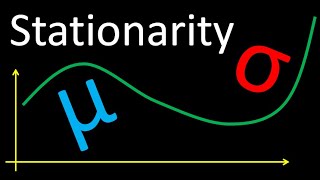
Today we are diving into an essential concept in time series analysis: stationarity. So, what is stationarity? Essentially, it's when the statistical properties of a time series, like the mean and variance, do not change over time.

Can you give an example of a stationary series?
Great question! An example of a stationary series could be the daily closing prices of a stock over time, if they show a consistent average price without observable trends or seasonality.

What about non-stationary data? What does that look like?
Non-stationary data often shows trends over time, like increasing average temperatures each year. This can lead to unreliable forecasts, which is why we check for stationarity.

Is there a way to tell if a series is stationary?
Yes, there are tests like the Augmented Dickey-Fuller test. It helps us determine if our time series has a unit root, meaning it's non-stationary.

That's interesting! How can we make a non-stationary series stationary?
We can use methods like differencing or log transformations to stabilize the mean and variance. Remember the acronym DLD: Differencing, Log transformation, Detrending.
To wrap up, stationarity ensures we work with reliable data. We test for it using methods like the ADF and KPSS tests, and transform non-stationary data through differencing, logging, or detrending.
Types of Stationarity
🔒 Unlock Audio Lesson
Sign up and enroll to listen to this audio lesson

Now, let's explore the types of stationarity. Who can tell me about strict stationarity?
I think strict stationarity means all statistical properties remain constant!
Exactly! Very well put. Strict stationarity means that not only the mean and variance but all moments of the distribution remain unchanged over time. Now, does anyone know the difference with weak stationarity?
Weak stationarity has constant mean and variance, but the entire distribution doesn't have to be the same?
Correct! Weak stationarity allows for the statistical properties to depend on time in a limited way, specifically through their covariance structure. Remember this: **W for Weak** = *Mean and Variance Stable*.
How do we decide which type of stationarity is needed for our analysis?
Great question! Usually, we aim for weak stationarity because it's sufficient for most time series modeling techniques. Understanding both types is crucial for model selection.
In summary, strict stationarity is more stringent, while weak stationarity is flexible and sufficient for analysis. Keep in mind the key differences when analyzing your data!
Testing for Stationarity
🔒 Unlock Audio Lesson
Sign up and enroll to listen to this audio lesson
Now, let’s focus on testing for stationarity. Can anyone name a test we can use?
The Augmented Dickey-Fuller test?
Absolutely! The ADF test checks for unit roots in a series. If we confirm a unit root, we conclude our data is non-stationary.
What about the KPSS test? How does that work?
Very good! The KPSS test has a different approach. Its null hypothesis states that the series is stationary. If our test statistic is greater than the critical value, we reject the null hypothesis, indicating non-stationarity.
That’s interesting! Are these tests used together?
Yes, they often complement each other. We might use the ADF test to confirm if there's a unit root, and then check with KPSS to validate if it’s stationary. This combination is helpful for robust analysis.
In summary, the ADF test determines if a unit root exists, while the KPSS test assesses the null hypothesis of stationarity. Utilizing these tests together can strengthen our findings.
Introduction & Overview
Read summaries of the section's main ideas at different levels of detail.
Quick Overview
Standard
This section discusses the concept of stationarity in time series data, outlining its types, how to test for it, and transformations that can be applied to achieve stationarity. Understanding stationarity is vital for ensuring reliable forecasts in time series models.
Detailed
Stationarity in Time Series
Stationarity is a key concept in time series analysis, indicating that the statistical properties of a dataset, such as the mean and variance, remain constant over time. Understanding whether a time series is stationary or non-stationary significantly impacts the forecasting accuracy.
Types of Stationarity
- Strict Stationarity: A time series is strictly stationary if its statistical properties are the same across all time periods—meaning that the entire distribution is unchanged over time.
- Weak Stationarity (Wide-sense): A time series is weakly stationary if its mean and variance are constant over time, and the covariance between two points depends only on the lag between them and not on the actual time at which the series is observed.
Testing for Stationarity
- Augmented Dickey-Fuller (ADF) Test: A common statistical test to check the null hypothesis that a unit root is present in a series, implying non-stationarity.
- KPSS Test: Tests the null hypothesis that a time series is stationary around a deterministic trend.
Transformations for Non-stationary Series
If a time series is found to be non-stationary, it can often be transformed into a stationary series through:
- Differencing: Calculating the difference between consecutive observations.
- Log Transformation: Applying the logarithmic function can help stabilize variance.
- Detrending: Removing trends from the data can also lead to stationarity.
In summary, stationarity is a critical component of time series analysis that must be established before fitting forecasting models. A clear understanding of the types, testing methods, and transformation techniques to achieve stationarity ensures that forecasts are grounded on reliable statistical assumptions.
Youtube Videos

Audio Book
Dive deep into the subject with an immersive audiobook experience.
Definition of Stationarity
Chapter 1 of 4
🔒 Unlock Audio Chapter
Sign up and enroll to access the full audio experience
Chapter Content
Stationarity means that the statistical properties of the series (mean, variance, autocorrelation) do not change over time.
Detailed Explanation
Stationarity in a time series indicates that its statistical characteristics remain constant over time. This definition includes key properties like the mean (the average value), variance (the degree of variation from the mean), and autocorrelation (the relationship between values at different times) being stable. When these properties do not change, it makes the data easier to model and predict.
Examples & Analogies
Think of a calm lake, where the surface remains flat and unchanging over time. This stability represents a stationary time series. In contrast, if you imagine a stormy ocean with waves constantly changing, that represents a non-stationary series with varying statistical properties.
Types of Stationarity
Chapter 2 of 4
🔒 Unlock Audio Chapter
Sign up and enroll to access the full audio experience
Chapter Content
Types:
• Strict Stationarity
• Weak Stationarity (Wide-sense)
Detailed Explanation
There are two main types of stationarity. Strict stationarity means the entire distribution of the time series remains unchanged over time. This is a more comprehensive and stringent requirement. On the other hand, weak stationarity, also known as wide-sense stationarity, only requires that the mean and variance are constant over time, and that the covariance between any two time points depends only on the time distance between them, not on the actual time. Weak stationarity is often sufficient for time series modeling.
Examples & Analogies
Imagine a clock ticking in a consistent rhythm; this represents weak stationarity where the intervals (mean) between ticks do not change. Meanwhile, a pendulum swinging in various arcs over time represents strict stationarity, where the behavior remains unchanged but requires every aspect (distribution) to remain uniform.
Testing for Stationarity
Chapter 3 of 4
🔒 Unlock Audio Chapter
Sign up and enroll to access the full audio experience
Chapter Content
Testing for Stationarity:
• Augmented Dickey-Fuller (ADF) Test
• KPSS Test
Detailed Explanation
To determine if a time series is stationary, we can use statistical tests. The Augmented Dickey-Fuller (ADF) Test checks for unit roots, which indicates non-stationarity. If the test result shows no unit root, the series is likely stationary. The KPSS Test (Kwiatkowski-Phillips-Schmidt-Shin) tests the null hypothesis that a series is stationary. If the test rejects this null hypothesis, it suggests non-stationarity. These tests provide a quantitative measure to assess stationarity, aiding in deciding how to model the data effectively.
Examples & Analogies
Consider these tests like scans used in hospitals. An ADF Test acts like an X-ray to check for problems in the structural integrity (unit roots) of a series, while the KPSS Test acts like a blood test, ensuring everything works smoothly (stationarity). The combination allows for a full health check of your time series.
Transforming Non-Stationary Series to Stationary
Chapter 4 of 4
🔒 Unlock Audio Chapter
Sign up and enroll to access the full audio experience
Chapter Content
Non-stationary series can often be transformed to stationary using:
• Differencing
• Log Transformation
• Detrending
Detailed Explanation
To convert non-stationary series into stationary ones, several methods can be utilized. Differencing involves subtracting the previous observation from the current one, which often stabilizes the mean. Log transformation can reduce variance and make relationships more linear. Detrending removes trends from the data to focus on stationary behavior. These techniques help prepare the data for modeling by ensuring that key statistical properties remain unchanged over time.
Examples & Analogies
Think of these transformations like preparing ingredients for cooking. Differencing is like slicing vegetables to ensure even cooking (stabilizing values), log transformation is akin to diluting a strong sauce for balanced flavor (reducing variance), and detrending is like removing excess fat from meat, allowing the main flavors to shine through (focusing on the core data).
Key Concepts
-
Stationarity: The property of a time series being invariant to time.
-
Strict Stationarity: All properties of the distribution are the same over any time period.
-
Weak Stationarity: Only the mean and variance are constant; covariance can depend on the time.
-
Testing for Stationarity: Uses statistical tests like ADF and KPSS.
-
Transforming to Stationarity: Methods include differencing, log transformation, and detrending.
Examples & Applications
A stock price that fluctuates around a constant mean value could indicate stationarity.
Monthly rainfall data that shows a trend upward over the years may be a non-stationary series.
Memory Aids
Interactive tools to help you remember key concepts
Rhymes
If the mean's the same all through, stationary’s for you!
Stories
Imagine a perfectly calm pond; if you drop a stone in, the ripples start to spread but settle back to calm. That’s the concept of stationarity!
Memory Tools
Remember the acronym DLD for transforming non-stationary data: D for Differencing, L for Log Transform, and D for Detrending.
Acronyms
STAY for STAtistical Year-round, meaning we're testing to see if properties STAY the same over time!
Flash Cards
Glossary
- Stationarity
A condition where the statistical properties of a time series, such as mean and variance, remain constant over time.
- Strict Stationarity
A type of stationarity where the entire distribution of the time series remains unchanged over time.
- Weak Stationarity
A type of stationarity where only the mean and variance of a time series are constant and the covariance depends on the lag.
- Augmented DickeyFuller Test (ADF)
A statistical test used to check for unit roots in a time series, indicating whether it is stationary.
- KPSS Test
A statistical test that assesses whether a time series is stationary around a deterministic trend.
- Differencing
A method for transforming a non-stationary series into a stationary one by calculating the difference between consecutive terms.
- Log Transformation
A method used to stabilize variance in time series data by applying a logarithmic function.
- Detrending
The process of removing trends from data to achieve stationarity.
Reference links
Supplementary resources to enhance your learning experience.