
Time and Space Complexity
Interactive Audio Lesson
Listen to a student-teacher conversation explaining the topic in a relatable way.
Understanding Time Complexity
🔒 Unlock Audio Lesson
Sign up and enroll to listen to this audio lesson

Welcome class! Today, we will explore time complexity. Can anyone tell me why we care about how long an algorithm takes to run?

I think it’s important because faster algorithms help our programs run better!
Exactly! We want our software to be efficient. Time complexity mainly deals with how the run time of an algorithm increases relative to the size of the input. Let’s discuss the common time complexities we use to measure this. What do you think constant time O(1) means?

That means the algorithm takes the same time no matter how big the input is, right?
Correct! For example, accessing an element in an array is O(1). Now, what about O(log n)?

That's for algorithms like binary search, which divides the problem in half each time!
Great job! The ability to halve the search space makes binary search very efficient. Let’s summarize: O(1) is constant time, while O(log n) shows more efficiency with increasing data, right?

Yes, and we also need to grasp that O(n) represents linear growth!
Diverse Examples of Time Complexity
🔒 Unlock Audio Lesson
Sign up and enroll to listen to this audio lesson

Now that we understand the basic complexities, let’s look at some examples. Can one of you explain O(n) with a real-life example?
Sure! If I have to search through a list of items one by one, that’s linear search which is O(n).
Exactly! Now, what about an example of O(n²)?
Bubble sort! It compares each element with every other element.
Spot on! It’s poor for large datasets due to its quadratic time complexity. How about we move on to space complexity?
Space Complexity
🔒 Unlock Audio Lesson
Sign up and enroll to listen to this audio lesson
Let’s shift gears to discuss space complexity. What does space complexity measure?
It measures how much memory an algorithm uses as the input size changes.
Exactly! Space complexity is vital in scenarios where memory is constrained. Can anyone give an example of an algorithm with high space complexity?
Recursive algorithms typically consume more stack space as they require additional memory for each call.
Correct! Understanding both time and space complexities enables us to make smarter decisions when selecting algorithms. Let’s summarize: Time complexity assesses how fast an algorithm runs, and space complexity evaluates how much memory it uses.
Introduction & Overview
Read summaries of the section's main ideas at different levels of detail.
Quick Overview
Standard
This section discusses the concepts of time complexity and space complexity with examples of various algorithms. It highlights how these complexities influence program performance and resource usage, providing a framework for understanding efficiency in software development.
Detailed
Time and Space Complexity
Time and space complexity are crucial metrics to evaluate the efficiency of algorithms. They represent the amount of time an algorithm takes to run and the amount of memory it consumes, respectively.
Time Complexity
- Constant Time (O(1)): The time taken is independent of the input size. For example, accessing an array element takes constant time.
- Logarithmic Time (O(log n)): The time grows logarithmically as the input size increases. An example is the binary search, which is highly efficient for sorted arrays.
- Linear Time (O(n)): The time taken grows linearly with the input size. The linear search algorithm exemplifies this complexity.
- Linearithmic Time (O(n log n)): This complexity is optimal for comparison-based sorts, such as merge sort and quick sort on average.
- Quadratic Time (O(n²)): Time increases quadratically with input size. Algorithms like bubble sort and selection sort fall into this category and are inefficient for large datasets.
- Exponential Time (O(2ⁿ), O(n!)): These algorithms are very inefficient for large inputs, often seen in advanced backtracking algorithms and permutations.
Space Complexity
Space complexity defines the memory required by an algorithm as its input size grows. Understanding both time and space complexity helps in selecting the right algorithms and data structures for specific application needs.
Youtube Videos


Audio Book
Dive deep into the subject with an immersive audiobook experience.
Understanding Time Complexity
Chapter 1 of 3
🔒 Unlock Audio Chapter
Sign up and enroll to access the full audio experience
Chapter Content
Time complexity affects how fast the program runs.
Detailed Explanation
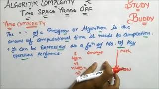
Time complexity is a way of representing the amount of time that an algorithm takes to complete as a function of the size of its input. This helps us to understand if an algorithm will be efficient or not. For example, an algorithm that runs in constant time, denoted as O(1), will take the same amount of time to execute regardless of the size of the input. In contrast, an algorithm that runs in linear time, O(n), will take time proportional to the size of the dataset — if the input doubles, so does the time.
Examples & Analogies
Think of time complexity like a car traveling a distance. If it's a flat road (constant time, O(1)), the car reaches the destination in the same amount of time, irrespective of whether there's one or more passengers (the input size). If it’s hilly (linear time, O(n)), for every additional mile you go, it takes a bit longer and you feel the strain with more stops, just like the algorithm takes longer as the input size increases.
Understanding Space Complexity
Chapter 2 of 3
🔒 Unlock Audio Chapter
Sign up and enroll to access the full audio experience
Chapter Content
Space complexity affects how much memory it uses.
Detailed Explanation
Space complexity measures the amount of memory an algorithm needs to run relative to the size of the input data. This is crucial because an algorithm could have a fast execution time but require excessive memory, which can lead to inefficient performance. For instance, an algorithm that uses O(n) space means that the memory requirement increases linearly with the input size. In contrast, O(1) denotes that the algorithm uses a constant amount of memory regardless of input size.
Examples & Analogies
Imagine you're packing for a trip. If your suitcase has a fixed size (constant space, O(1)), it doesn’t matter if you pack a few items or many; the space remains limited. However, if you have a backpack that can expand to fit all your clothes (linear space, O(n)), then the more items you add, the more space you need — similar to how an algorithm's memory usage grows with the size of its input.
Performance Classes of Algorithms
Chapter 3 of 3
🔒 Unlock Audio Chapter
Sign up and enroll to access the full audio experience
Chapter Content
Complexity Example Algorithm Performance (n = size of input)
- O(1) Accessing array element Constant time
- O(log n) Binary search Very efficient
- O(n) Linear search Scales linearly
- O(n log n) Merge sort, Quick sort (avg) Optimal for comparison-based sorts
- O(n²) Bubble/Selection sort Poor for large datasets
- O(2ⁿ), O(n!) Recursive backtracking, permutations Very inefficient.
Detailed Explanation
Different algorithms have distinct performance characteristics, often expressed using 'Big O' notation. Here's a breakdown of some common classes:
1. O(1): Accessing a specific item in an array takes the same time regardless of the array size, offering quick access.
2. O(log n): Algorithms like binary search are efficient for sorted data, significantly reducing the time needed as the data set grows.
3. O(n): Linear search scans items one by one; its performance directly scales with input size.
4. O(n log n): Advanced sorting algorithms like Merge Sort combine linear and logarithmic elements, which is optimal for comparison-based sorting in practice.
5. O(n²): Algorithms like Bubble Sort are inefficient for large datasets due to their quadratic growth in performance.
6. O(2ⁿ), O(n!): These represent factorial growth and become practically unfeasible very quickly, often encountered in complex recursive functions.
Examples & Analogies
Consider a library. O(1) is like walking straight to a specific book on the shelf—it takes the same time no matter how big the library is. O(log n) is like a librarian using a catalog to find books efficiently without looking at every single row. O(n) is similar to searching every shelf sequentially—it works but takes longer as the library grows. O(n log n) is like organizing books in batches, which is smart but needs more preparation time. O(n²) is like checking every book against every other book—super tedious. O(2ⁿ) or O(n!) is like trying to compare every possible arrangement of a book order for a massive collection; incredibly overwhelming!
Key Concepts
-
Time Complexity: Indicates how the execution time of an algorithm scales with the input size.
-
Space Complexity: Refers to the amount of memory an algorithm needs during execution.
-
O(1): Represents constant time operations.
-
O(log n): Signifies logarithmic time efficiency, often used in searching algorithms.
-
O(n): Denotes linear time complexities, common in straightforward algorithms.
Examples & Applications
Accessing an element in an array has O(1) time complexity since it doesn't depend on the input size.
Binary search has a time complexity of O(log n) and is efficient for sorted arrays.
Memory Aids
Interactive tools to help you remember key concepts
Rhymes
For algorithms that rush, O(1) does not fuss; it's quick as a hush, with no input crush.
Stories
Imagine a librarian who sorts books by title. If she checks only the first book each time, it's O(1). If she opens each book to find the correct one, it’s O(n).
Memory Tools
For remembering time complexities: C, L, Log, Q - C is for constant, L is linear, Log is logarithmic, and Q is for quadratic.
Acronyms
T S O (Time, Space, Order) - helps you recall the assessment factors for algorithms.
Flash Cards
Glossary
- Time Complexity
A measure of the amount of computational time that an algorithm takes to complete as a function of the input size.
- Space Complexity
The amount of memory space required by an algorithm to execute as a function of the input size.
- O(1)
Constant time complexity where the execution time doesn’t depend on the input size.
- O(log n)
Logarithmic time complexity indicating that the execution time increases logarithmically with input size.
- O(n)
Linear time complexity indicating that the execution time grows linearly with input size.
- O(n²)
Quadratic time complexity which indicates that execution time grows proportionally to the square of the input size.
Reference links
Supplementary resources to enhance your learning experience.