
Complex Exponentials and Fourier Analysis
Interactive Audio Lesson
Listen to a student-teacher conversation explaining the topic in a relatable way.
Introduction to Complex Exponentials
🔒 Unlock Audio Lesson
Sign up and enroll to listen to this audio lesson

Today, we're diving into complex exponentials. These are important because they can represent sinusoidal functions. Can anyone tell me what a sinusoidal function looks like?

Is that like a sine or cosine wave?
Exactly! A sinusoidal function can be expressed using complex exponentials thanks to Euler’s formula: $e^{j heta} = ext{cos}( heta) + j ext{sin}( heta)$. This helps us analyze signals in different domains.

So, complex exponentials help us break down signals?
Yes! They allow us to represent signals in a more manageable form. Remember: **'E for Exponential and S for Sinusoid'**. That’s our mnemonic!

Can you give an example of how we use that?
Of course! For instance, we can express a signal like $x(t) = A e^{j 2 au f t}$ and analyze it using its frequency components.
Fourier Transform Overview
🔒 Unlock Audio Lesson
Sign up and enroll to listen to this audio lesson

Now, let's talk about the Fourier Transform. Who can explain what it does?

It transforms signals from the time domain to the frequency domain, right?
Correct! The Fourier transform gives us a way to express a signal as a sum of sinusoids. The mathematical representation is $X(f) = \int_{-\infty}^{\infty} x(t) e^{-j 2 \pi f t} dt$. What do you think is the significance?
Maybe it helps us understand what frequencies are present in a signal?
Absolutely! This is crucial in signal processing for tasks such as filtering and compression. Remember our acronym: **'F for Frequency'**.
Discrete Fourier Transform (DFT)
🔒 Unlock Audio Lesson
Sign up and enroll to listen to this audio lesson
Let’s switch gears to the Discrete Fourier Transform. What is it for?
It analyzes discrete signals in the frequency domain, right?
Yes! And it’s defined as $X[k] = \sum_{n=0}^{N-1} x[n] e^{-j 2 \pi \frac{k n}{N}}$. Why might we use the DFT instead of the Fourier transform?
Because we often work with sampled data?
Exactly! The DFT is specifically designed for analyzing signals that are already in a discrete form. Let’s remember: **'D for Discrete and F for Fast'** since we often use the Fast Fourier Transform algorithm to compute it.
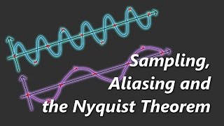
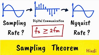
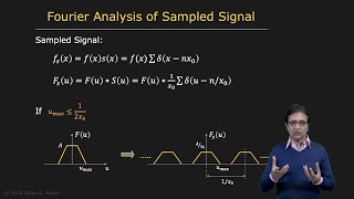
Sampling Theorem and Its Connection to Fourier Analysis
🔒 Unlock Audio Lesson
Sign up and enroll to listen to this audio lesson
Finally, let’s connect everything with the sampling theorem. Who can remind us what the Nyquist-Shannon theorem states?
We need to sample at least twice the highest frequency of the signal to avoid aliasing.
Yes! If we sample at a lower rate, what happens?
We get aliasing, where high frequencies interfere with the lower frequencies.
Exactly! It's vital to understand this relationship between sampling and frequency content through Fourier analysis. Let’s use a mnemonic: **'S for Sampling and C for Content'** to remember.
Introduction & Overview
Read summaries of the section's main ideas at different levels of detail.
Quick Overview
Standard
Complex exponentials and Fourier analysis serve as crucial mathematical tools in signal processing, allowing us to decompose signals into their frequency components. By expressing signals using complex exponentials and applying the Fourier transform, we gain insights into the behavior of signals in both continuous and discrete domains.
Detailed
Detailed Summary of Complex Exponentials and Fourier Analysis
In this section, we explore two fundamental concepts in digital signal processing: complex exponentials and Fourier analysis. Complex exponentials are defined as signals of the form
$$ x(t) = A e^{j 2 au f t} $$
where A is the amplitude, f is frequency, t is time, and j is the imaginary unit. Using Euler’s formula, complex exponentials can be split into sinusoidal signals, which are the building blocks of many real-world signals.
Next, we delve into the Fourier transform, a powerful mathematical tool used to convert a continuous-time signal into its frequency-domain representation. The Fourier transform of a signal x(t) is given by the integral
$$ X(f) = \int_{-\infty}^{\infty} x(t) e^{-j 2 \pi f t} dt $$
This representation allows us to analyze the frequency components, providing a deeper understanding of signal behavior.
Furthermore, we introduce the Discrete Fourier Transform (DFT), which is used for analyzing discrete signals. The DFT is defined mathematically as
$$ X[k] = \sum_{n=0}^{N-1} x[n] e^{-j 2 \pi \frac{k n}{N}} $$
where N is the number of samples, and k indicates the frequency index. The DFT facilitates efficient computation using the Fast Fourier Transform (FFT) algorithm, a critical component in modern signal processing.
The relationship between the sampling theorem and Fourier analysis shows that proper sampling preserves the signal's frequency content. Understanding these relationships is vital to avoiding aliasing and ensuring accurate signal reconstruction.
Youtube Videos
Audio Book
Dive deep into the subject with an immersive audiobook experience.
Introduction to Complex Exponentials
Chapter 1 of 5
🔒 Unlock Audio Chapter
Sign up and enroll to access the full audio experience
Chapter Content
Complex exponentials and Fourier analysis are fundamental tools in signal processing, enabling us to represent signals in the frequency domain and understand their frequency content. These concepts are central to both continuous and discrete-time signal analysis.
Detailed Explanation
This chunk introduces the significance of complex exponentials and Fourier analysis in signal processing. Complex exponentials allow us to represent signals mathematically in the frequency domain. Essentially, when we talk about signals, we often need to analyze their behavior not just over time, but also understand what frequencies are present within them. By transforming signals into the frequency domain, we can simplify the processes involved in analyzing, filtering, and reconstructing these signals.
Examples & Analogies
Consider a music composer who pieces together various melodies and harmonies (signals). To understand how each sound contributes to the overall music (frequency content), they might break down the song into notes (frequencies). Just like understanding the structure of music helps in creating better compositions, analyzing signals in the frequency domain helps in better signal processing.
Understanding Complex Exponentials
Chapter 2 of 5
🔒 Unlock Audio Chapter
Sign up and enroll to access the full audio experience
Chapter Content
A complex exponential is a signal of the form:
x(t)=Aej2πft
Where:
- A is the amplitude.
- f is the frequency.
- t is time.
- j is the imaginary unit.
This complex exponential signal can be decomposed into its real and imaginary components using Euler’s formula:
ejθ=cos(θ)+jsin(θ)
Thus, a complex exponential can represent sinusoidal signals, which are the building blocks of all signals.
Detailed Explanation
Complex exponentials help in representing signals that oscillate, such as sound waves or radio waves. They are generally described in the form x(t)=Aej2πft, where A gives us the amplitude (how strong the signal is), and f indicates the frequency (how many cycles occur in a second). Euler’s formula breaks down the complex exponential into sine and cosine functions, which are critical in studying oscillatory behavior. This makes complex exponentials valuable for representing varying signals in a way that is mathematically manageable.
Examples & Analogies
Think of complex exponentials as a waveform of light. Just as light can be broken down into different colors (wavelengths) that we can see (visible spectrum), complex exponentials provide a way to decompose signals into their fundamental waves (sine and cosine), helping us understand the overall structure of the signal.
Fourier Transform Overview
Chapter 3 of 5
🔒 Unlock Audio Chapter
Sign up and enroll to access the full audio experience
Chapter Content
The Fourier transform is a mathematical tool used to convert a continuous-time signal x(t) from the time domain into the frequency domain. The Fourier transform expresses the signal as a sum of sinusoids (complex exponentials), providing a frequency representation of the signal. The Fourier transform of a continuous-time signal x(t) is given by:
X(f)=∫−∞∞x(t)e−j2πft dt
Where:
- X(f) is the frequency-domain representation of the signal.
- x(t) is the time-domain signal.
- f is the frequency.
Detailed Explanation
The Fourier transform enables us to see how different frequency components are present within a signal. Specifically, it transforms the signal from time-based analysis (where we look at how the signal changes over time) to frequency-based analysis (where we look at how much of each frequency is present). The mathematical expression shows that we integrate (sum up) all the contributions from the sine and cosine components at various frequencies to get a complete 'map' of frequency content in the signal.
Examples & Analogies
Imagine you have a fruit salad (signal) mixed with bananas, apples, and grapes (different frequencies). If you want to know how many pieces of each fruit there are (frequency content), you would have to sort through the salad to count each type of fruit. The Fourier transform is like that sorting process, converting a complex mix of flavors (time domain signal) into identifiable categories (frequency domain representation).
Discrete Fourier Transform (DFT)
Chapter 4 of 5
🔒 Unlock Audio Chapter
Sign up and enroll to access the full audio experience
Chapter Content
The Discrete Fourier Transform (DFT) is used to analyze discrete-time signals in the frequency domain. The DFT is defined as:
X[k]=∑n=0N−1x[n]e−j2πknN
Where:
- x[n] is the discrete-time signal.
- X[k] is the DFT of the signal.
- N is the number of samples.
- k is the frequency index.
Detailed Explanation
The DFT takes a finite set of sample points from a signal and converts them into their frequency components. It performs a similar function to the Fourier transform but is specifically designed for discrete data, allowing for frequency analysis of signals that have been digitized and sampled. The equation summarizes this transformation and demonstrates how each sample contributes to the overall frequency representation.
Examples & Analogies
Think of the DFT as a recipe that requires a specific number of ingredients (samples). If you’re baking cookies, the DFT helps you understand how the different flavors combine to create the overall taste (frequency content) of the cookie, allowing you to appreciate what each ingredient contributes to the final product.
Sampling Theorem Connection
Chapter 5 of 5
🔒 Unlock Audio Chapter
Sign up and enroll to access the full audio experience
Chapter Content
Fourier analysis and the sampling theorem are closely related. The sampling theorem ensures that when we sample a continuous-time signal, the signal's frequency components are preserved, provided the sampling rate exceeds twice the maximum frequency in the signal. The Fourier transform helps us analyze how signals are represented in the frequency domain, providing insights into the behavior of the signal after sampling. When sampling, the frequency components of the continuous signal are replicated at multiples of the sampling frequency, which is known as spectral folding.
Detailed Explanation
The sampling theorem, primarily known for guiding how often we need to sample signals to accurately capture their essence, ties directly into Fourier analysis. It states that if we sample at a rate greater than twice the highest frequency in the signal, we can recover the original signal without distortion. When sampled improperly (too low a rate), frequency components can overlap, leading to aliasing. Fourier analysis aids in visualizing these frequency components, thus giving us a clearer picture of potential problems and solutions.
Examples & Analogies
Imagine you are taking pictures of a moving object. If you take a photo every second (sampling rate), but the object moves quickly (high frequency), you might miss shapes and details. The Nyquist theorem ensures you capture enough frames (samples) to represent the object accurately, just like sampling ensures we capture frequency information completely to avoid any ambiguity in the final analysis.
Key Concepts
-
Complex Exponential: A function that can represent sinusoidal signals.
-
Fourier Transform: Converts time-domain signals into their frequency-domain representation.
-
Discrete Fourier Transform (DFT): Analyzes finite-length discrete signals.
-
Sampling Theorem: Ensures proper sampling to avoid aliasing.
-
Aliasing: Distortion due to insufficient sampling rates.
Examples & Applications
Example of a complex exponential: x(t) = 5 e^{j 2 au 1000 t}, representing an amplitude of 5 and frequency of 1000 Hz.
The Fourier transform of a rectangular pulse signal can yield a sinc function in the frequency domain, indicating its frequency spread.
Memory Aids
Interactive tools to help you remember key concepts
Rhymes
Fourier's magic, sinusoids unfold, in the frequency domain, the secrets told.
Stories
Imagine a musician tuning their instruments; each note corresponds to a frequency, revealing its essence through transformation.
Memory Tools
Remember 'S for Sampling, C for Content' to recall the sampling theorem.
Acronyms
InFFT
Inverse Fourier is Fast Transform to remember DFT.
Flash Cards
Glossary
- Complex Exponential
A function of the form x(t) = A e^{j 2 au f t}, representing sinusoidal signals.
- Fourier Transform
A mathematical transform that expresses a time-domain signal as a sum of sinusoids in the frequency domain.
- Discrete Fourier Transform (DFT)
A transformation used to analyze discrete-time signals in the frequency domain, computed efficiently via the Fast Fourier Transform algorithm.
- Sampling Theorem
A principle stating that a continuous-time signal can be perfectly reconstructed from its samples if sampled at a rate greater than twice its highest frequency.
- Aliasing
The distortion that occurs when high-frequency components of a signal are misrepresented due to insufficient sampling rates.
Reference links
Supplementary resources to enhance your learning experience.