
Estimation of Mixing Height
Enroll to start learning
You’ve not yet enrolled in this course. Please enroll for free to listen to audio lessons, classroom podcasts and take practice test.
Interactive Audio Lesson
Listen to a student-teacher conversation explaining the topic in a relatable way.
Introduction to Mixing Height and Lapse Rates
🔒 Unlock Audio Lesson
Sign up and enroll to listen to this audio lesson

Today we'll start discussing mixing height, which is crucial for understanding how pollutants disperse in the air. Can anyone tell me what you think mixing height means?

Is it the height at which pollutants mix with the surrounding air?
Exactly! Mixing height is where the pollutants become well-mixed with the atmosphere. Now, can anyone explain what lapse rates are?

I think lapse rates are about how temperature changes with altitude, right?
Correct! There are two main types: the environmental lapse rate, which can vary, and the dry adiabatic lapse rate, which is a theoretical constant, approximately -9.8 degrees Celsius per kilometer. Let's keep these in mind.

How does that relate to pollutant transport?
Great question! The interaction between these two lapse rates helps determine if conditions are unstable, stable, or neutral.
To summarize, we learned about mixing height's importance in atmospheric science and how lapse rates help us understand temperature changes with altitude.
Effects of Stability on Pollutant Transport
🔒 Unlock Audio Lesson
Sign up and enroll to listen to this audio lesson

Let's explore how stability affects pollutant transport. Who remembers what we mean by unstable conditions?
Unstable conditions are when the environmental lapse rate is greater than the adiabatic lapse rate?
Exactly! In such conditions, pollutants can rise and disperse widely. What about stable conditions?

In stable conditions, the environmental lapse rate is less than the adiabatic lapse rate, which makes pollutants tend to stay below the mixing height.
Spot on! This situation can lead to increased pollution concentration at the ground level. Why is this important?
It means pollution can affect health more in stable conditions.
Great insight! To summarize, we've identified how unstable and stable conditions influence pollutant dispersion based on mixing height.
Measurement and Calculation of Mixing Height
🔒 Unlock Audio Lesson
Sign up and enroll to listen to this audio lesson
Now, let's learn how to estimate the mixing height. Can anyone explain how we gather the necessary data?
We can measure the environmental lapse rate by using balloons, right?
Yes! Balloons can provide temperature profiles as they rise. What do we then do with the data?
We compare the environmental lapse rate with the adiabatic lapse rate.
Precisely! The intersection of these two rates gives us the mixing height. Why is it important for us to understand this?
It helps us predict how pollutants will behave in the atmosphere.
Exactly! Understanding these calculations allows us to anticipate pollution levels and their impact on health. Summarizing today, we discussed how to gather and use data to estimate mixing height, linking it to the dispersion of pollutants.
Plume Behavior and Mixing Height
🔒 Unlock Audio Lesson
Sign up and enroll to listen to this audio lesson
Let's talk about plume behavior in relation to mixing height. Can anyone name one type of plume behavior?
There's looping, where the plume goes up and down.
Correct! Looping happens in unstable conditions. What about other types?
Coning occurs when the environmental lapse rate is about the same as the adiabatic lapse rate.
Yes! In coning, the plume spreads more uniformly. How does that affect pollutant concentration?
Less concentration at the ground, right?
Exactly! This is important for understanding air quality and its implications for public health. So, we have discussed several plume behaviors and their role in pollutant dispersion.
Summary and Real-World Applications of Mixing Height
🔒 Unlock Audio Lesson
Sign up and enroll to listen to this audio lesson
In our final session, let's reflect on the real-world implications of mixing height. Why is this knowledge critical for cities?
It helps in understanding how to manage air quality.
Exactly, managing air quality is vital for public health. Cities can use this information to implement better pollution control measures. Can anyone think of an example?
Like restricting vehicle emissions in high pollution zones?
Right! Regulations can be adjusted based on the mixing height and the associated pollution levels. To summarize our discussions, we have covered the significance of mixing height, how to calculate it, the various plume behaviors, and the real-world applications of these concepts.
Introduction & Overview
Read summaries of the section's main ideas at different levels of detail.
Quick Overview
Standard
The section elaborates on the concept of mixing height, which is crucial for understanding pollutant dispersion in the atmosphere. It presents various atmospheric stability conditions and how they affect the transport of pollutants, focusing on measurement methods for environmental and adiabatic lapse rates.
Detailed
Estimation of Mixing Height
In this section, we explore the estimation of mixing height (MMH) as a vital component in the dispersion of pollutants in the atmosphere. Mixing height is influenced significantly by the environmental lapse rate and the adiabatic lapse rate. When studying pollutant transport, understanding the conditions of stability—whether unstable, neutral, or stable—is essential. In unstable conditions, with high mechanical turbulence and a rapid drop in temperature with height, pollutants can mix more effectively.
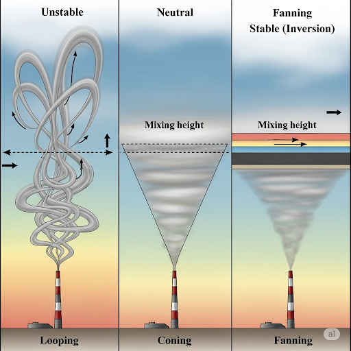
The section explains how to calculate the mixing height by measuring the environmental lapse rate, which varies daily and seasonally, usually through balloon releases to obtain temperature profiles. The dry adiabatic lapse rate is a fixed theoretical value, while the actual adiabatic lapse rate may differ based on local conditions. Different plume behaviors influenced by mixing height, such as looping, coning, fanning, fumigation, lofting, and trapping, showcase the complexity of pollutant dispersion depending on the environmental conditions, particularly regarding temperature inversions. Understanding these interactions helps predict pollutant behaviors in various atmospheric conditions.
Youtube Videos


Audio Book
Dive deep into the subject with an immersive audiobook experience.
Understanding Mixing Height
Chapter 1 of 4
🔒 Unlock Audio Chapter
Sign up and enroll to access the full audio experience
Chapter Content
So, sometimes you have to calculate the mixing height. The estimation of mixing height is simply this you have to take the environmental lapse rate at that point and the adiabatic lapse rate.
Detailed Explanation
Mixing height is a crucial factor in understanding how pollutants disperse in the atmosphere. To estimate mixing height, you need to consider two types of lapse rates: the environmental lapse rate and the adiabatic lapse rate. The environmental lapse rate indicates how temperature changes with height in the atmosphere, while the adiabatic lapse rate reflects how the temperature of a rising air parcel changes, usually at a theoretical rate of about -9.8 degrees Celsius per kilometer. By analyzing where these two rates intersect, you can determine the mixing height.
Examples & Analogies
Imagine trying to figure out the point at which hot air from a lamp mixes with cooler air in a room. The ‘mixing height’ is like the height where the hot air meets the cooler air and starts to mix rather than sitting separately. Just as you’d consider the temperature change as you move away from the lamp to understand that mixing, scientists measure temperature changes in the atmosphere to pinpoint where pollution might disperse.
Measurement of Lapse Rates
Chapter 2 of 4
🔒 Unlock Audio Chapter
Sign up and enroll to access the full audio experience
Chapter Content
Let us say that you have some scenario like this. So, which means I need environmental lapse rate the temperature profile is measured on a daily basis usually.
Detailed Explanation
Meteorological departments often monitor the temperature of the atmosphere by sending balloons that measure temperatures at different heights. This data provides a daily record of temperature profiles and helps derive the environmental lapse rate specific to a particular location. Understanding these profiles is essential as they can change due to weather conditions, influencing the mixing height.
Examples & Analogies
Think of how chefs taste food at various stages of cooking—this helps them determine the perfect flavor at the end. Similarly, meteorologists collect temperature readings at various heights to ‘taste’ the atmosphere, allowing them to understand how pollutants will disperse and mix based on the environmental conditions.
Estimation Errors in Mixing Height
Chapter 3 of 4
🔒 Unlock Audio Chapter
Sign up and enroll to access the full audio experience
Chapter Content
So, you have to understand one thing that because there is a lot of fluctuation, lot of error in this kind of estimations it is very difficult to estimate this accurately.
Detailed Explanation
Estimating mixing height can be complicated due to the fluctuations in temperature and atmospheric conditions. This variability often leads to errors in the estimated height where mixing occurs. Moreover, while ideal values (like the dry adiabatic lapse rate of -9.8°C/km) can provide guidance, real-world conditions may deviate significantly from these estimates due to environmental factors such as humidity or changing weather patterns.
Examples & Analogies
Imagine trying to predict the best time for a picnic based only on the weather forecast—sometimes, the prediction may not account for sudden rain showers or wind changes. Just like in weather predictions, estimating mixing heights can involve uncertainties, with many factors influencing the final outcome.
Sources of Pollution
Chapter 4 of 4
🔒 Unlock Audio Chapter
Sign up and enroll to access the full audio experience
Chapter Content
If you have a point source, you know exactly what the temperature is and where it is and all that what the height is, but if you have an area or line source for a road for example...
Detailed Explanation
When dealing with pollution sources, it is essential to understand the nature of the source. Point sources, like a single factory chimney, allow for precise temperature measurements of the emissions. In contrast, line sources, such as roads, produce emissions along a continuous path, making it challenging to pinpoint specific temperatures or emissions at any single point. These variations can affect how pollutants mix in the atmosphere.
Examples & Analogies
Consider a fountain that shoots water straight up—this is like a point source, easy to measure and predict. Now think about a garden hose spraying water all along its length; it’s much more complex to know exactly how each droplet behaves. Pollution works the same way; knowing the type of source helps determine how pollutants behave in the air.
Key Concepts
-
Mixing Height: The critical altitude for effective mixing of pollutants.
-
Lapse Rates: Rates indicating temperature variation with height, affecting stability.
-
Plume Behavior: Describes how pollutant plumes behave under various atmospheric conditions.
Examples & Applications
During a summer day with high instability, pollutants can rise significantly, increasing air quality concerns.
During nighttime inversions, pollutants can become trapped near the ground, leading to higher concentrations.
Memory Aids
Interactive tools to help you remember key concepts
Rhymes
Mixing height, don't delay, keep pollutants from going astray.
Stories
Imagine a hot air balloon rising; the heat causes pollutants to dance and swirl within the mixing height, spreading evenly. But when the balloon descends into cooler air, the dance stops, and the pollutants stagnate, causing pollution to stay close to the ground.
Memory Tools
HATS: Height, Adiabatic, Turbulence, Stability - to remember factors affecting pollutant dispersion.
Acronyms
MHT
Mixing Height Theory - includes concepts of lapse rates and their roles in dispersion.
Flash Cards
Glossary
- Mixing Height
The height at which pollutants become well-mixed with the surrounding atmosphere.
- Environmental Lapse Rate
The rate at which the temperature of the atmosphere decreases with an increase in altitude.
- Adiabatic Lapse Rate
The theoretical rate of temperature decline with altitude under dry adiabatic conditions, generally -9.8°C per kilometer.
- Turbulence
The chaotic and irregular motion of air that aids in mixing pollutants in the atmosphere.
- Plume
The visible trail of pollutants emitted from a source, taking shape based on atmospheric conditions.
Reference links
Supplementary resources to enhance your learning experience.