
Gaussian Dispersion Model - Example, Additional topics
Enroll to start learning
You’ve not yet enrolled in this course. Please enroll for free to listen to audio lessons, classroom podcasts and take practice test.
Interactive Audio Lesson
Listen to a student-teacher conversation explaining the topic in a relatable way.
Understanding the Gaussian Dispersion Model
🔒 Unlock Audio Lesson
Sign up and enroll to listen to this audio lesson

Let's delve into the Gaussian Dispersion Model. It’s used extensively for estimating pollutant concentrations from sources like industrial stacks. Can anyone tell me why this model is important?

I think it helps us understand how pollutants spread into the environment.
Exactly, it helps predict how different factors, such as wind and atmospheric stability, affect pollution distribution. This understanding can aid in environmental safety. Remember the acronym SOLAR for Sources, Observations, Locations, Atmosphere, and Receptors — these are key elements.

So it’s crucial for planning industrial sites too?
Yes! Proper site planning can minimize exposure risks. The model gives a preliminary handle on potential impacts.

What happens if there are multiple sources?
Great question! All emissions can be added together, allowing us to assess cumulative effects effectively.

So, if I wanted to visualize this, how would I draw it?
You can create a contour map showing varying pollutant concentrations around sources, like isopleths. To summarize, the model is invaluable for predicting and managing air quality.
Calculating Concentrations
🔒 Unlock Audio Lesson
Sign up and enroll to listen to this audio lesson

Let's now apply the model to calculate sulfur dioxide concentrations at specific points. Who recalls the concentrations we are estimating?
We’re looking at 50 and 500 meters from the stack, right?
Correct! The stack is 60 meters high and emanates 160 grams per second of SO2. We also need to consider atmospheric stability. How do we determine the stability class?
We use data from tables based on weather conditions.
Exactly! Stability influences how pollutants disperse. For instance, stability class D—which we’ll use—implies moderate conditions. Can anyone tell me the key parameters needed for the calculations?
We need sigma values for both vertical and horizontal dispersion!
Right! These values depend on the distance from the source and the stability class. Remember to apply these correctly during calculations.
What was the concentration value we calculated earlier?
You’re referring to the concentration at 500 meters; it was 66 micrograms per meter cubed. To recap, we estimate values using our dispersion parameters and stability classes.
Real-World Applications
🔒 Unlock Audio Lesson
Sign up and enroll to listen to this audio lesson
Now that we understand the calculations, let’s discuss real-world applications. How could the data from our emissions model be useful?
It could guide emergency responses in case of hazardous leaks.
Exactly, emergency planners need precise data to identify potentially affected areas. What’s another way this model is beneficial?
It helps in selecting industrial sites away from population centers.
Correct! Avoiding residential areas minimizes health risks. Anyone recall the types of non-idealities the model doesn't account for?
Stack tip downwash, where emissions can recirculate due to low pressure?
Exactly! And building downwash impacts emissions spread around large buildings. It’s critical to be aware of these artifacts when interpreting data.
So how do these issues affect our calculations?
These factors can lead to higher local concentrations than predicted. Thus, accurate modeling and site assessments are key. In summary, the Gaussian model forms a fundamental part of environmental impact assessments.
Introduction & Overview
Read summaries of the section's main ideas at different levels of detail.
Quick Overview
Standard
The section explores the application of the Gaussian Dispersion Model by providing a detailed example of estimating SO2 concentrations at different distances from a stack. It discusses stability classes, factors affecting dispersion, and the significance of accurate measurements in environmental assessments.
Detailed
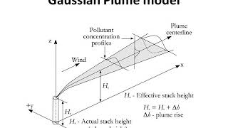
The Gaussian Dispersion Model is essential for estimating pollutant concentrations from emission sources such as stacks. This section begins with a practical example to assess the ground-level concentration of sulfur dioxide (SO2) emissions at 50 and 500 meters from a stack of 60 meters in height, emitting 160 grams per second. The calculations involve determining factors such as the stability class of the atmosphere, which can vary the resulting concentration values due to natural variability in conditions and assumptions. Students are guided through deriving concentration values at different points while acknowledging the model's idealism and associated non-idealities, such as stack tip downwash and building downwash. The significance of accurate pollutant distribution mapping is highlighted, especially concerning emergency response planning and industrial site selection. The integration of multiple source emissions adds complexity but is manageable through the model, emphasizing the need for precise coordinates and meteorological inputs for effective environmental monitoring and analysis.
Youtube Videos


Audio Book
Dive deep into the subject with an immersive audiobook experience.
Estimating SO2 Concentration
Chapter 1 of 11
🔒 Unlock Audio Chapter
Sign up and enroll to access the full audio experience
Chapter Content
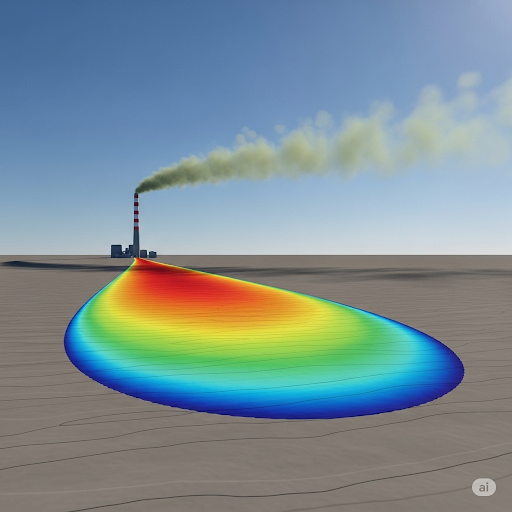
So we want to look at SO2 emission from a stack. So this is what we want, estimate SO2 concentration at ground level center line 50 and 500 meters from the stack. So there is a stack here and we are looking at a distance 500 meters from the stack and we want to know, what is the concentration? Center line at ground level which means y equals to 0, z equals 0.
Detailed Explanation
This part discusses how to estimate sulfur dioxide (SO2) concentration from an emission stack, focusing specifically on two distances: 50 meters and 500 meters from the stack. The concentration is assessed at ground level, defined by y=0 (crosswind position) and z=0 (vertical position). Essentially, this steps into the practical application of the Gaussian dispersion model, which assumes that pollutants disperse symmetrically from the source.
Examples & Analogies
Imagine you're standing at a barbecue grill, and you want to know how strong the smoke is at different distances. You can measure the smoke intensity right next to the grill (0 meters), 50 meters away, and then further at 500 meters. Just like tracking the smoke, this model calculates how a pollutant like SO2 spreads from its source.
Stability Class and Parameters
Chapter 2 of 11
🔒 Unlock Audio Chapter
Sign up and enroll to access the full audio experience
Chapter Content
From the overcast conditions, we can select the stability class from the Pascal differs table so for slight insulation stability class is D.
Detailed Explanation
In this section, stability classes are referenced, particularly class D for slight insulation conditions. The stability class is important as it reflects how stable the atmosphere is at the time of emission. A stability class indicates how well air can mix; class A (very stable) means less mixing, while class D (slightly unstable) allows for a moderate amount of dispersion, making it critical for calculating pollutant concentrations accurately.
Examples & Analogies
Think about how the weather works: on a calm day, the air feels heavy and stagnant (class A), while on a breezy day, the air mixes well and disperses heat and odors more effectively (class D). The stability class in dispersion modeling works similarly, indicating how much mixing and dispersing happens in the atmosphere.
Calculating Sigma Values
Chapter 3 of 11
🔒 Unlock Audio Chapter
Sign up and enroll to access the full audio experience
Chapter Content
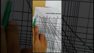
We are looking at x equals 500, so it means that the computation of σ at x equals 500 will take this is 500 meters. We go to stability class D. This line is stability class D and then I pick my value for σ as 36 meters there and similarly I do this for σ also at the 500.
Detailed Explanation
In Gaussian models, 'sigma' (σ) represents the standard deviation of the pollutant concentration distribution. This part explains how to compute the sigma values at a distance of 500 meters from the stack. By using stability class D, the calculated sigma values help establish how wide the pollutant plume will be as it disperses. Essentially, the greater the sigma value, the wider the plume, leading to lower concentrations at a specific point.
Examples & Analogies
Imagine throwing a handful of seeds from a height. The wider you throw them, the more scattered they'll get below. In our case, sigma is like the spread of those seeds; a larger sigma means the SO2 is more spread out at 500 meters, reducing the concentration.
Calculating Pollutant Concentration
Chapter 4 of 11
🔒 Unlock Audio Chapter
Sign up and enroll to access the full audio experience
Chapter Content
And I get a value of 66 microgram meter cube of SO2. This is the concentration at that point.
Detailed Explanation
After calculating the parameters, the ultimate goal is to find the concentration of SO2 at a specific distance. Here, we determine that the concentration at 500 meters is 66 micrograms per cubic meter of air. This concentration helps evaluate the potential health risks associated with SO2 emissions and whether they exceed safety thresholds.
Examples & Analogies
Think of measuring how sweet a drink is. If you taste a sip (like going to a specific point downwind from the source), you can determine how much sugar (pollutant concentration) is present. In this model, we calculated how much SO2 is in the air at a distance, akin to tasting and measuring sweetness at different spots.
Crosswind Effects on Concentration
Chapter 5 of 11
🔒 Unlock Audio Chapter
Sign up and enroll to access the full audio experience
Chapter Content
Second example; so here we set 50 meters crosswind, which means that y is not 0 anymore, y is off the x axis 50 meters away.
Detailed Explanation
In this example, the analysis shifts to a crosswind position at 50 meters. The term 'crosswind' implies a position perpendicular to the direction of the wind. Here, understanding how pollutants behave not just downwind but also sideways is essential to build a comprehensive air quality model. The distance enhances the model's accuracy by providing feedback on how pollutants disperse across various points around the emission source.
Examples & Analogies
If you stand by a fountain and feel the mist, you notice some droplets land much further away, especially if the wind blows. This illustrates how pollutants can also drift side-to-side, not just straight downwind, showing how dispersion happens in multiple directions.
Multiple Source Contributions
Chapter 6 of 11
🔒 Unlock Audio Chapter
Sign up and enroll to access the full audio experience
Chapter Content
For example, if you are interested in doing a large number of sources, I am looking at a top view of a map there is a source here, we call it source 1, the source 1 has plume... all of these 3 will contribute to concentration here.
Detailed Explanation
When analyzing air quality, it's important to consider multiple emission sources rather than just one. Each source releases pollutants that can all overlap or combine at a particular location. This explains how to add the contributions from each source to get a total concentration at a given point. This integrated perspective is essential for comprehensive air quality management.
Examples & Analogies
Think of a busy intersection where several cars are honking. Each car adds its noise (pollution) to the overall sound level. By looking at it this way, you can better understand the total noise impact just like combining emissions from multiple sources helps measure total air pollution levels.
Grid of Receptors for Measurement
Chapter 7 of 11
🔒 Unlock Audio Chapter
Sign up and enroll to access the full audio experience
Chapter Content
The application when we do this we define a grid of measurement coordinates also called as receptors.
Detailed Explanation
To measure pollutant concentrations effectively, we create a grid system known as receptors. These specific coordinates help track concentration levels across various points, enhancing the analysis of air quality over an area. The reference frame allows us to categorize emissions according to geographical distribution and ascertain how pollutants affect different regions.
Examples & Analogies
Imagine placing a series of microphones around a concert hall to measure sound levels at different spots. Similarly, receptors are strategically placed locations that help ascertain the pollutant levels in their vicinity and give a clearer picture of air quality.
Visual Representation of Pollution Data
Chapter 8 of 11
🔒 Unlock Audio Chapter
Sign up and enroll to access the full audio experience
Chapter Content
The way we do it is by mapping it... what is called an isopleth? An isopleth is the line joining points of equal concentration, so this gives you a contour map.
Detailed Explanation
Once data is collected from the receptors, the next step is visualization. The concept of isopleths makes it possible to create contour maps, where lines join equal levels of pollutant concentration. These maps serve as a visual tool in understanding how pollution spreads and allows for targeted analysis regarding air quality issues in specific areas.
Examples & Analogies
Similar to how weather maps show areas of rain or sunshine using contour lines, pollution maps illustrate where concentrations are high or low. For instance, a contour map showing pollution levels around a factory can quickly reveal the areas severely affected by emissions.
Emergency Response Planning
Chapter 9 of 11
🔒 Unlock Audio Chapter
Sign up and enroll to access the full audio experience
Chapter Content
What this application gives you is; let us say that 50 milligrams per meter cube is the ambient exposure level you cannot anything above 50 is supposed to be not safe.
Detailed Explanation
Understanding the concentration of pollutants helps in emergency response planning. By identifying regions where concentrations exceed safety thresholds, planners can establish boundaries for hazard exposure. Immediate actions can be defined to protect public health, especially during accidents or emergencies involving hazardous materials.
Examples & Analogies
Think of a fire drill in a school. If alarms go off above a certain threshold (like pollution levels), teachers guide students to safe zones. Similarly, in real-life scenarios, knowing pollution hotspots allows authorities to instruct residents on safety measures quickly, like evacuation if necessary.
Industrial Site Planning
Chapter 10 of 11
🔒 Unlock Audio Chapter
Sign up and enroll to access the full audio experience
Chapter Content
The second type of application in sense how you can use this information is to plan this sighting of industry.
Detailed Explanation
By utilizing dispersion modeling, industries can be strategically placed in locations that minimize adverse health effects on surrounding populations. By assessing wind patterns and potential emission impacts, planners can decide optimal locations for new industries, ensuring that emissions impact areas with the least population density.
Examples & Analogies
Imagine planning a picnic. You’d choose a park far away from busy roads to avoid pollution. Likewise, urban planners and industries need to strategically site factories in less populated areas to reduce exposure to harmful emissions.
Non-Idealities in Dispersion Modeling
Chapter 11 of 11
🔒 Unlock Audio Chapter
Sign up and enroll to access the full audio experience
Chapter Content
There are a couple of small Artifacts to this dispersion, these are the non-idealities one of them is called as stack tip downwash...
Detailed Explanation
Non-idealities such as stack tip downwash and building downwash refer to situations where emission dispersion does not behave as the Gaussian model predicts. These phenomena create low-pressure regions that can lead to high pollutant concentrations at ground level, especially nearby sources. Understanding these non-idealities is crucial for accurate air quality assessments.
Examples & Analogies
Think about how wind flows around obstacles like trees or buildings. Just as smoke can swirl back down or linger due to a building, pollutants can similarly be trapped, leading to unhealthy air quality for people nearby.
Key Concepts
-
Dispersion modeling is essential for predicting how pollutants spread and impact air quality.
-
Calculating pollutant concentration requires understanding stability classes and meteorological conditions.
-
Multiple emissions can be assessed collectively to evaluate overall air quality impacts.
-
Non-idealities, such as stack tip and building downwash, can affect concentration predictions.
Examples & Applications
Assessing sulfur dioxide concentrations at various distances from a stack to understand emission impacts.
Using contour maps to visualize pollutant concentrations around industrial sites, assisting in emergency response planning.
Memory Aids
Interactive tools to help you remember key concepts
Rhymes
Pollutants spread in the air, where wind goes, they don't care!
Stories
Imagine a stack in a busy city, releasing smoke. Depending on the wind's mood, that smoke drifts high or low, swirling around buildings like a dance until it settles or dissipates.
Memory Tools
Remember SOAR for the Gaussian model: Sources, Observations, Area, and Receptors.
Acronyms
STACK
Stability
Temperature
Area Coordinates
and Kinetics for dispersion modeling.
Flash Cards
Glossary
- Gaussian Dispersion Model
A mathematical model used to predict the concentration of pollutants in the atmosphere, considering factors like wind speed and atmospheric stability.
- Stability Class
Categories that indicate the atmospheric conditions affecting pollutant dispersion, commonly classified from A (very stable) to D (moderately unstable).
- Concentration
The amount of substance (pollutant) per unit volume, typically measured in micrograms per cubic meter (µg/m³).
- Pollutant
Any substance that, when introduced into the environment, causes adverse effects to human health or ecosystems.
- Stack Height
The vertical distance from the ground to the top of a stack or chimney, impacting how pollutants disperse.
Reference links
Supplementary resources to enhance your learning experience.