
Least Mean Squares (LMS) Algorithm
Interactive Audio Lesson
Listen to a student-teacher conversation explaining the topic in a relatable way.
Introduction to LMS Algorithm
🔒 Unlock Audio Lesson
Sign up and enroll to listen to this audio lesson

Today, we're exploring the Least Mean Squares, or LMS, algorithm. Can anyone tell me what they think this algorithm does?

Is it something to do with making predictions based on data?
Exactly, Student_1! The LMS algorithm adjusts filter coefficients to minimize the mean square error between the desired target and the output of the filter. Remember the acronym MSE for mean square error—this will help you remember its goal!

How does it update those filter coefficients?
Great question! The update rule is crucial. It follows the formula: w[n+1] = w[n] + μe[n]x[n], where w represents the filter coefficients, μ is the step size, and e is the error signal. We can remember this rule as a way of gradually adjusting our predictions!
Understanding the Update Rule
🔒 Unlock Audio Lesson
Sign up and enroll to listen to this audio lesson

Now, let’s focus on the update rule of the LMS algorithm. Can someone explain what each component represents?

The w[n] is the current coefficients, right? And e[n] is the difference between the desired output and the predicted output?
Correct! e[n] = d[n] - y^[n] gives us the error signal. And what about x[n]?

It’s the input signal at that time, I think?
Exactly! Understanding each component is vital, especially when choosing the step size μ. It's like tuning an instrument; too high and it can be unstable, too low and it takes too long to adapt. Why do you think this might be important?
If the adaptation is too slow, it won't work well in situations where conditions change rapidly, like in real-time audio processing.
Convergence of the LMS Algorithm
🔒 Unlock Audio Lesson
Sign up and enroll to listen to this audio lesson
Let’s discuss convergence. What do you all understand by this term in machine learning?
I think it's how quickly an algorithm can find the best solution?
Absolutely! In LMS, if the step size μ is chosen incorrectly, it can either lead to oscillations or make the algorithm take forever to find its optimal point. Can anyone think of a situation where this might be a problem?
In real-time communication like VoIP, if it can't quickly adapt to changes, the call quality could suffer.
Exactly, Student_3! So, balancing adaptation speed and stability is vital in applications like speech processing or noise cancellation.
Applications of the LMS Algorithm
🔒 Unlock Audio Lesson
Sign up and enroll to listen to this audio lesson
Now, let’s explore where the LMS algorithm is used practically. Can anyone name an application?
Noise cancellation! I think it's used in headphones.
Correct! It’s widely applied for noise cancellation. What other areas can you think of?
Maybe in equalization for cellular signals?
Exactly! Adaptive filters using LMS help equalize signals to improve communication quality. Remember the versatility of these algorithms in dynamic environments!
Introduction & Overview
Read summaries of the section's main ideas at different levels of detail.
Quick Overview
Standard
The LMS algorithm efficiently updates filter coefficients to minimize the mean square error (MSE) through an iterative process. Its adaptability makes it a popular choice in dynamic environments, crucial for applications ranging from noise cancellation to prediction.
Detailed
Least Mean Squares (LMS) Algorithm
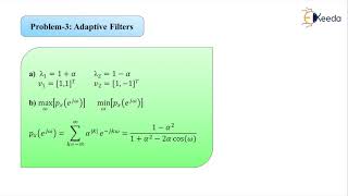
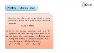
The Least Mean Squares (LMS) algorithm is one of the foundational techniques in the design of adaptive filters. It operates primarily by minimizing the Mean Square Error (MSE) between a desired output signal and the actual output generated by an adaptive filter. The algorithm achieves this by updating filter coefficients iteratively based on the input signal and the calculated error.
Key Points:
- Update Rule: The LMS algorithm employs a specific update rule for filter coefficients, expressed as:
$$ w[n+1] = w[n] + \mu e[n] x[n] $$
where: - $w[n]$ is the filter coefficient vector at time $n$.
- $\mu$ is the step-size parameter which influences the adaptation speed.
- $e[n]$ is the error signal calculated by the difference between the desired output and the actual adaptive filter output.
- $x[n]$ is the input signal at time $n$.
- Convergence: The convergence of the LMS algorithm significantly depends on the step-size parameter $\mu$. A well-chosen $\mu$ balances adaptation speed with stability, and is often chosen through experimentation or theoretical analysis.
- Simplicity and Efficiency: The LMS algorithm is favored for its low computational cost and quick convergence relative to other adaptive algorithms, making it particularly suitable for real-time applications.
The ability to tune adaptive filters using the LMS algorithm underlies its application in various fields, including noise cancellation, echo cancellation, prediction in time-series data, and system identification.
Youtube Videos

Audio Book
Dive deep into the subject with an immersive audiobook experience.
Overview of the LMS Algorithm
Chapter 1 of 4
🔒 Unlock Audio Chapter
Sign up and enroll to access the full audio experience
Chapter Content
The Least Mean Squares (LMS) algorithm is one of the simplest and most widely used algorithms for adaptive filter design. The LMS algorithm minimizes the mean square error (MSE) between the desired output and the filter's output by iteratively updating the filter coefficients.
Detailed Explanation
The LMS algorithm forms the backbone of many adaptive filtering applications. Its core objective is to reduce the difference between the output we want (the desired output) and what the filter actually produces. This difference is referred to as the mean square error (MSE). The process of minimizing this error is accomplished through a systematic adjustment of the filter parameters or coefficients, making the LMS algorithm an essential tool in signal processing.
Examples & Analogies
Think of the LMS algorithm like a student trying to refine their essay. Initially, the essay may not fully meet the teacher’s expectations (the desired output). The student receives feedback (the error signal) indicating where they need to improve. With each rewrite (iteration), they adjust their content to reduce the feedback, ultimately achieving a refined version that aligns with what the teacher wanted.
LMS Algorithm Update Rule
Chapter 2 of 4
🔒 Unlock Audio Chapter
Sign up and enroll to access the full audio experience
Chapter Content
The LMS algorithm updates the filter coefficients w[n] using the following equation:
w[n+1] = w[n] + μe[n]x[n]
Where:
● w[n] is the vector of filter coefficients at time n.
● μ is the step-size parameter, controlling the rate of adaptation.
● e[n]=d[n]−y^[n] is the error signal, with d[n] as the desired output.
● x[n] is the input signal at time n.
Detailed Explanation
The update rule for the LMS algorithm is a mathematical formula that describes how the filter coefficients need to be adjusted to improve accuracy over time. Each coefficient is updated based on the product of the error signal (the discrepancy between what we want and what we have) and the current input signal. The step-size parameter (μ) controls how large each adjustment should be: a smaller value leads to more stability but slower learning, while a larger value can speed up learning at the risk of stability.
Examples & Analogies
Consider a sailor adjusting their sails based on wind direction. The error signal acts like measuring how well the current sail setup is catching the wind (desired output), while the sailor tweaks the sail's position (filter coefficients) based on the immediate wind feedback (input signal). The step-size is like the sailor's responsiveness; if they make small adjustments, they stabilize their ship well but might not catch all the wind quickly.
Convergence of LMS
Chapter 3 of 4
🔒 Unlock Audio Chapter
Sign up and enroll to access the full audio experience
Chapter Content
The convergence of the LMS algorithm depends on the step-size parameter μ. If μ is too large, the algorithm may become unstable and fail to converge. If μ is too small, convergence will be slow. The optimal value of μ is often chosen experimentally or based on theoretical analysis.
Detailed Explanation
Convergence in the context of the LMS algorithm refers to how quickly and reliably the algorithm finds the right filter coefficients that minimize the error signal. If the step-size parameter (μ) is set too high, the filter can overreact to any fluctuations, leading to instability, where the coefficients oscillate without settling. Conversely, if μ is too low, the adjustments made are minimal, resulting in a very slow approach to achieving the desired performance. Finding a balanced μ is crucial for effective adaptation.
Examples & Analogies
Imagine trying to tune a radio. If you turn the dial too quickly, you might skip over the channel entirely (unstable). But if you turn it too slowly, it takes ages to get to the station you want (slow convergence). The trick is to find a speed that lets you smoothly and quickly adjust to the right station.
Advantages of the LMS Algorithm
Chapter 4 of 4
🔒 Unlock Audio Chapter
Sign up and enroll to access the full audio experience
Chapter Content
The LMS algorithm is known for its simplicity, low computational cost, and relatively fast convergence, making it a popular choice for adaptive filtering tasks.
Detailed Explanation
The LMS algorithm is favored in many applications due to its straightforward implementation and efficiency. Its simplicity means that it requires less computational power compared to more complex algorithms, making it suitable for real-time processing scenarios. Additionally, the relatively fast convergence allows it to adapt quickly to changing conditions, which is vital in dynamic environments.
Examples & Analogies
Think of the LMS algorithm as a basic recipe for cooking. It doesn’t require fancy ingredients or complex cooking techniques (low computational cost), making it accessible for many home cooks. While there are more gourmet dishes that take longer to prepare and require more skill, many people appreciate being able to whip up a quick, tasty meal that still satisfies (fast convergence and efficiency).
Key Concepts
-
LMS Algorithm: An adaptive filtering method to minimize mean square error.
-
Mean Square Error (MSE): The average of the square differences between estimated and actual values.
-
Filter Coefficient Update: The iterative process to adjust coefficients to optimize performance.
-
Convergence: The ability of the algorithm to reach stability under adaptation.
Examples & Applications
In noise cancellation systems, the LMS algorithm can effectively adapt to different noise environments, providing clearer audio experiences.
In financial forecasting, the LMS algorithm can predict stock prices by adjusting to market changes.
Memory Aids
Interactive tools to help you remember key concepts
Rhymes
LMS adjusts, it takes its cue, to minimize the error that isn't true.
Stories
Imagine a chef who tastes their soup repeatedly. If it's too salty, they add water. This is like the LMS algorithm adjusting its filter coefficients based on the error signal until the soup is just right!
Memory Tools
Remember LMS: "Least Mistakes Signal;" this reflects its goal of reducing error.
Acronyms
LMS - Learn, Minimize, Signal. Focuses on learning from input to minimize errors in signal processing.
Flash Cards
Glossary
- Least Mean Squares (LMS)
An adaptive filtering algorithm that minimizes the mean square error by iteratively updating filter coefficients.
- Mean Square Error (MSE)
A measure of the average squared difference between the estimated values and the actual value.
- Filter Coefficients
Parameters in an adaptive filter that determine the filter's output based on the input signal.
- Error Signal
The difference between the desired output and the actual output, used for adjusting filter coefficients.
- StepSize Parameter (μ)
A value that controls the rate of adaptation in the LMS algorithm.
Reference links
Supplementary resources to enhance your learning experience.