Finite Impulse Response (FIR) filters are a class of digital filters with a finite number of coefficients. FIR filters are widely used in digital signal processing (DSP) due to their inherent stability and simplicity in implementation. A common and simple example of an FIR filter is the Moving Average Filter, which is widely used for smoothing signals and reducing noise. In this chapter, we will explore the concept of FIR filters, focusing on the Moving Average Filter, its properties, design, and applications.

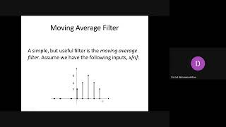
A Moving Average Filter (MAF) is a specific type of FIR filter that calculates the output as the average of the most recent NN input samples. It is widely used for smoothing signals, reducing noise, and performing simple signal averaging. The moving average filter is one of the simplest FIR filters to implement. The equation for an N-point Moving Average Filter is:

y[n]=1N∑k=0N−1x[n−k]

Let’s consider a simple example where we apply a 3-point moving average filter to the following input signal x[n]:
x[n]={5,10,15,20,25,30}.
To compute the output y[n] for each sample, we use the moving average equation with N=3. The output at each time step is the average of the current and the two previous samples.

FIR filters, including the moving average filter, have several important properties that make them useful in digital signal processing:
1. Linear Phase: FIR filters can be designed to have a linear phase response, meaning that all frequency components of the signal are delayed by the same amount.
2. Stability: FIR filters are always stable because their impulse response is finite.
3. Implementation Simplicity: FIR filters are easy to implement because they do not require feedback and only use a finite number of coefficients.
4. No Feedback: FIR filters are non-recursive, meaning that they do not rely on previous output values.

The frequency response of an FIR filter defines how it modifies the amplitude and phase of different frequency components of the input signal. For a moving average filter, its frequency response depends on the filter length NN. The frequency response H(f) of an FIR filter can be found by computing the Discrete Fourier Transform (DFT) of the filter coefficients.

FIR filters, including moving average filters, can be designed for a wide variety of applications, from noise reduction to frequency response shaping. The design process typically involves:
1. Choosing the Desired Frequency Response: The desired cutoff frequency and shape of the filter's frequency response must be defined based on the application.
2. Selecting the Filter Length NN: The filter length determines the number of samples used to compute the moving average.
3. Windowing Methods: The design of FIR filters often involves windowing techniques.
4. Computing Filter Coefficients: The filter coefficients can be calculated using techniques such as the frequency sampling method, Parks-McClellan algorithm, or window method.

1. Noise Reduction: Moving average filters are often used to reduce high-frequency noise from signals.
2. Signal Smoothing: In applications like ECG or EEG signal processing, moving average filters are used to smooth the signal.
3. Edge Detection in Image Processing: Moving average filters can also be used in image processing to detect edges.
4. Real-Time Data Processing: Moving average filters are used in real-time data processing for applications like temperature control.

The Moving Average Filter (MAF) is one of the simplest and most widely used FIR filters in digital signal processing. It is effective for tasks like smoothing signals, reducing noise, and performing simple signal averaging. As a member of the FIR filter family, the moving average filter benefits from properties like stability and linear phase, making it a valuable tool in many applications.