
Thornwaite-Holzman Equation
Enroll to start learning
You’ve not yet enrolled in this course. Please enroll for free to listen to audio lessons, classroom podcasts and take practice test.
Interactive Audio Lesson
Listen to a student-teacher conversation explaining the topic in a relatable way.
Introduction to the Thornwaite-Holzman Equation
🔒 Unlock Audio Lesson
Sign up and enroll to listen to this audio lesson

Today, we're diving into the Thornwaite-Holzman Equation. This equation helps us understand how moisture content changes in the soil can affect emission flux. Who can explain what emission flux means?

Isn't it the rate at which moisture or other gases are released from a surface?
Exactly! As moisture in the soil varies, the partition constant changes, influencing the overall flux. Can anyone recall what a partition constant is?

I think it's the ratio of the concentration of a substance in two phases, like soil and air.
That's correct! Understanding these fundamentals is crucial as we move on.
Understanding Flux Measurement Techniques
🔒 Unlock Audio Lesson
Sign up and enroll to listen to this audio lesson

Now let's talk about flux measurement techniques, particularly the gradient technique. Why do we use it?

We use it when it's hard to enclose a surface to measure flux.
Right! And this technique relies on measuring concentration at different heights. Why is that important?

It helps us understand how concentration gradients vary vertically!
Exactly! The concentration differences allow us to calculate the flux. Can anyone summarize how turbulence impacts these measurements?
Turbulence creates fluctuations in mass transfer, which complicates measuring gradients but is essential to consider.
Well put! Let's remember the turbulence's role as we delve deeper.
Application of Friction Velocity
🔒 Unlock Audio Lesson
Sign up and enroll to listen to this audio lesson
Next, let's focus on friction velocity. Can anyone tell me what it is?
It's shear stress at the surface divided by density.
Great! And how does it relate to the Thornwaite-Holzman Equation?
Friction velocity helps calculate velocity gradients which represent how quickly the airflow changes with height.
Exactly! Understanding these gradients is key to predicting how materials transport in turbulent conditions.
Introducing the Monin-Obukhov Length Scale
🔒 Unlock Audio Lesson
Sign up and enroll to listen to this audio lesson
Now let’s discuss the Monin-Obukhov length scale. Who can explain what it represents?
It measures the height scale at which turbulence production by buoyancy matches shear stress.
Exactly! It's crucial in modifying the Thornwaite-Holzman Equation when thermal forces come into play. Why is accounting for thermal effects important?
Because temperature gradients can significantly alter the flow and turbulence dynamics, affecting mass flux.
Absolutely! Integration of these principles leads us to a more accurate model of flux.
Introduction & Overview
Read summaries of the section's main ideas at different levels of detail.
Quick Overview
Standard
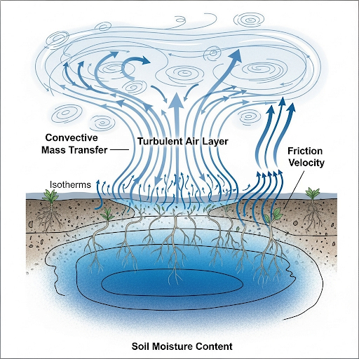
This section delves into the Thornwaite-Holzman Equation, illustrating how changes in moisture content and turbulence affect flux in soil and air. It also introduces the concepts of convective mass transfer, turbulent diffusion, and the significance of factors like friction velocity and the Monin-Obukhov length scale.
Detailed
Thornwaite-Holzman Equation
The Thornwaite-Holzman Equation is critical in understanding how mass transfer occurs in turbulent environments, particularly in soil and air. Moisture content in soil changes, affecting the partition constant and consequently the mass flux. This equation illustrates the correlations between concentration gradients, turbulence, and mass transfer in different atmospheric stability conditions.
Key Concepts:
- Moisture Content and Partition Constants: As moisture content changes in soil, the emission flux reacts dynamically. This section emphasizes the experimental data showcasing this relationship through models.
- Gradient Technique: When measuring flux in conditions where enclosure is impractical, a gradient or micrometeorological technique is employed. This technique utilizes concentration differences to gauge fluxes, capitalizing on turbulence and convective eddies.
- Convective Mass Transfer: This crucial part of understanding the Thornwaite-Holzman Equation includes analyzing vertical components of movement that influence concentration gradients, thereby affecting mass flux.
- Friction Velocity: Defined as shear stress over density, friction velocity is crucial for calculating velocity gradients and understanding turbulence at varying heights.
-
Monin-Obukhov Length Scale: This concept addresses the impact of thermal forces on turbulence and the resulting mass transfer dynamics, introducing factors such as stability depending on temperature gradients.
The section concludes with the derivation of a modified Thornwaite-Holzman equation that accounts for thermal influences, ultimately creating a more accurate estimation of flux in turbulent conditions.
Youtube Videos


Audio Book
Dive deep into the subject with an immersive audiobook experience.
Fundamentals of Soil Moisture and Flux
Chapter 1 of 8
🔒 Unlock Audio Chapter
Sign up and enroll to access the full audio experience
Chapter Content
So this is again the thing that we discussed in last class. When this kind of thing happens, moisture content in the soil is changing as a result emission will change. The partition constant is changing, this is changing.
Detailed Explanation
In this introduction, the relationship between soil moisture content and emission patterns is established. When moisture in the soil changes, it leads to alterations in the emission of chemicals, represented through the 'partition constant'. This indicates that as the conditions in the soil vary, the rates at which materials are emitted also shift, reflecting a dynamic interaction between the soil's physical state and its chemical behavior.
Examples & Analogies
Think about a sponge. When a sponge is dry, it doesn't release any water vapor. But once it absorbs water, it starts to release that moisture into the air. Similarly, when soil moisture content changes due to environmental factors, the same principles of absorption and emission apply.
Experiment and Observations
Chapter 2 of 8
🔒 Unlock Audio Chapter
Sign up and enroll to access the full audio experience
Chapter Content
This experiment is done in the lab where it shows that there is a chemical called dibenzofuran and this is experimental data. When the mud is dry and this is the model, the blue line is the model that shows, and then at some point we dry the surface by sending in dry air, okay. So the water content increases. The water flux increases because it is now being dried and then the water increase and then everything is dry.
Detailed Explanation
This chunk discusses a specific experiment involving dibenzofuran, showcasing its effects on mud when dry air is introduced. As dry air is blown across the mud surface, the moisture content is affected — specifically, the water content in the soil increases due to evaporation, leading to changes in water flux. The relationship between drying and moisture levels is pivotal in understanding how emissions from the soil are regulated.
Examples & Analogies
Imagine a desert where plants release moisture during hot, dry days. As the temperature rises, the moisture in the soil evaporates quickly, causing the plants to draw up more water from their roots. This constant cycle illustrates how drying conditions can amplify moisture loss and alter environmental emissions.
Measuring Flux in Open Surfaces
Chapter 3 of 8
🔒 Unlock Audio Chapter
Sign up and enroll to access the full audio experience
Chapter Content
When you have a surface and you have to measure the flux and it is difficult for you or it is unreliable for you to enclose a surface, you need to still measure the flux and we do it by what is called as a gradient technique or a micrometeorological technique.
Detailed Explanation
This chunk introduces the 'gradient technique' or 'micrometeorological technique' used to measure flux when enclosing a surface is impractical. It essentially involves measuring variations in concentration over a gradient to deduce flux. This method allows scientists to gather necessary data about emissions without needing to construct artificial environments, which is key in real-world field studies.
Examples & Analogies
Consider how weather forecasts are made by measuring temperatures and humidity at different heights above the ground. Just like these measurements help predict weather, the gradient technique helps scientists measure how different soil surfaces emit gases over various distances.
Understanding Convective Mass Transfer
Chapter 4 of 8
🔒 Unlock Audio Chapter
Sign up and enroll to access the full audio experience
Chapter Content
This is convective mass transfer right. This is convective mass transfer and therefore we are trying to take advantage of the convective mass transfer component in the z direction to see what is the concentration difference and we will also see if we can somehow measure the net flux based on that concentration difference at a given location.
Detailed Explanation
In this section, the text describes convective mass transfer, which refers to the moving flow of materials (like gases or vapors) due to differences in concentration. By assessing the vertical flow and concentration differences within this framework, researchers can determine how substances are transferring from soil surfaces into the air and measure the overall flux. This concept is essential for understanding how substances interact with the environment.
Examples & Analogies
Imagine cooking on a stove. As you heat water in a pot, the steam rises, creating a convection current. Similarly, when substances evaporate from soil, the movement of air influences how they disperse into the atmosphere, highlighting the importance of airflow in emission processes.
Deriving Flux Expressions
Chapter 5 of 8
🔒 Unlock Audio Chapter
Sign up and enroll to access the full audio experience
Chapter Content
So, we have measurements of concentration at two heights, velocity at two heights that will give us some idea of the structure v star, the turbulent structure of the thing, and then we are using these terms here.
Detailed Explanation
This chunk explains how measurements of concentration and velocity at two different heights can be utilized to derive expressions related to flux in an open environment. The concept of 'v star' is introduced, representing how turbulent structures influence the movement and concentration of emitted chemicals. Understanding these relationships is crucial for accurately predicting flux rates based on various environmental measurements.
Examples & Analogies
Think of a river flowing with varying depths. Measuring the flow at different points allows you to understand its overall behavior. Similarly, measuring concentrations and velocities at various heights helps scientists capture the more complex dynamics of how emissions behave in the atmosphere.
Impact of Stability on Flux
Chapter 6 of 8
🔒 Unlock Audio Chapter
Sign up and enroll to access the full audio experience
Chapter Content
When there is neutral condition, which means that there is no, neutral condition means stability is neutral, there is no thermal forces pushing up and down, no buoyancy effects, the terms and kinematic viscosity and diffusivity are assumed to be same.
Detailed Explanation
This chunk elaborates on the concept of 'neutral condition', where buoyancy effects are absent, meaning that thermal forces do not influence the flow of air. In this state, the characteristics of kinematic viscosity and diffusivity are seen as the same. This neutrality is crucial for simple calculations of flux, as it eliminates variables that can complicate predictions of material movement.
Examples & Analogies
Consider a calm day without wind — the air is stable, and everything behaves predictably. In such conditions, predicting the movement of scents from flowers is straightforward. However, on windy days, the movements become unpredictable, similar to how thermal conditions can complicate flux estimates.
Modification for Thermal Forces
Chapter 7 of 8
🔒 Unlock Audio Chapter
Sign up and enroll to access the full audio experience
Chapter Content
For that, there is something called as modified Thornwaite-Holzman equation. When you have thermal forces, you bring into this question. There is something called as a Monin-Obukhov length scale.
Detailed Explanation
Here, the text introduces the modified Thornwaite-Holzman equation, which incorporates thermal forces into flux calculations. The Monin-Obukhov length scale is introduced, serving as a critical factor to account for the effects that thermal forces have on turbulence and, ultimately, material flux rates. This adjustment is essential for accurate predictions when thermal effects are significant.
Examples & Analogies
Think about a balloon being warmed by the sun. The warmth causes the air inside to rise, influencing how the balloon floats and moves. Similarly, when thermal forces are at play in the atmosphere, they dramatically alter how emissions are dispersed from the ground.
Final Adjustments in Flux Calculation
Chapter 8 of 8
🔒 Unlock Audio Chapter
Sign up and enroll to access the full audio experience
Chapter Content
So based on this, we define a bunch of other things. So we add a correction factor called as Beta which is now dependent on the stability as well and this when we have a bunch of equations where we calculate Beta for different values.
Detailed Explanation
This final chunk discusses the introduction of a correction factor, called Beta, which adjusts calculations based on stability conditions. This factor is crucial for refining flux estimates, especially in situations where environmental factors affect dispersion. By using various equations tailored to different stability scenarios, scientists can enhance the accuracy of their emissions analyses.
Examples & Analogies
When baking, adjusting ingredients based on humidity and temperature alters the final product. Similarly, adding correction factors helps refine emission predictions based on environmental conditions. Without these adjustments, the results may be off, much like a cake that doesn't rise due to an inaccurate recipe.
Key Concepts
-
Moisture Content and Partition Constants: As moisture content changes in soil, the emission flux reacts dynamically. This section emphasizes the experimental data showcasing this relationship through models.
-
Gradient Technique: When measuring flux in conditions where enclosure is impractical, a gradient or micrometeorological technique is employed. This technique utilizes concentration differences to gauge fluxes, capitalizing on turbulence and convective eddies.
-
Convective Mass Transfer: This crucial part of understanding the Thornwaite-Holzman Equation includes analyzing vertical components of movement that influence concentration gradients, thereby affecting mass flux.
-
Friction Velocity: Defined as shear stress over density, friction velocity is crucial for calculating velocity gradients and understanding turbulence at varying heights.
-
Monin-Obukhov Length Scale: This concept addresses the impact of thermal forces on turbulence and the resulting mass transfer dynamics, introducing factors such as stability depending on temperature gradients.
-
-
The section concludes with the derivation of a modified Thornwaite-Holzman equation that accounts for thermal influences, ultimately creating a more accurate estimation of flux in turbulent conditions.
Examples & Applications
Example of moisture content affecting soil emission rates shows how drier conditions lead to lower flux.
Illustration of a gradient measurement technique, with air samples taken at two heights to evaluate flux based on concentration differences.
Memory Aids
Interactive tools to help you remember key concepts
Rhymes
Flux flows up when dryness takes hold, moisture's a keeper of secrets untold.
Stories
Imagine a garden where watered plants thrive. Measure their growth by watching how tall they strive, just as we measure flux, rising high when moisture takes flight.
Memory Tools
FLOP: Friction, Lateral movement, Outflow, Partition to remember key aspects of flux in the Thornwaite-Holzman Equation.
Acronyms
FLUX - Friction, Lateral, Upward, X-concentration gradients.
Flash Cards
Glossary
- ThornwaiteHolzman Equation
An equation that describes the relationship between the concentration gradient of a substance and its mass flux, accounting for turbulence effects.
- Emission Flux
The rate at which a substance is emitted from a surface into the atmosphere.
- Partition Constant
The ratio of a substance's concentration in two phases, such as soil and air.
- Gradient Technique
A measurement method used to determine flux by assessing concentration differences over heights without enclosing the surface.
- Friction Velocity
The velocity scale used in turbulence calculation, defined as the shear stress at the surface divided by the density.
- MoninObukhov Length Scale
A length scale that represents the height at which buoyancy effects equal shear stress, affecting atmospheric turbulence.
Reference links
Supplementary resources to enhance your learning experience.