
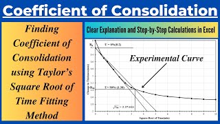
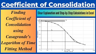
Log – time curve fitting method
Enroll to start learning
You’ve not yet enrolled in this course. Please enroll for free to listen to audio lessons, classroom podcasts and take practice test.
Interactive Audio Lesson
Listen to a student-teacher conversation explaining the topic in a relatable way.
Introduction to Log-Time Curve Fitting
🔒 Unlock Audio Lesson
Sign up and enroll to listen to this audio lesson

Today, we’re going to explore the Log-time curve fitting method, which helps us understand the consolidation of soils. Can anyone tell me why consolidation is important in engineering?

It shows how soils settle over time, right?
Exactly! And that’s why understanding how to determine the coefficient of consolidation, Cv, is crucial for construction projects. The Log-time curve fitting method uses a logarithmic scale to plot data effectively.

What does it mean to use a logarithmic scale?
Great question, Student_2! A logarithmic scale helps us manage a wide range of values more conveniently. It compresses the scale, making it easier to analyze long-term behavior of soil consolidation.

So it’s like squishing everything together to see the bigger picture?
Exactly! It allows us to identify trends effectively. Now, let's delve deeper into the steps of this method.
Steps in the Log-Time Curve Fitting Method
🔒 Unlock Audio Lesson
Sign up and enroll to listen to this audio lesson

Let’s go over the steps of the Log-time curve fitting method. First, we plot our dial readings against time using a logarithmic scale. Who can remind us why we plot time on a log scale?

It helps to visualize the data better, especially when the time values are very different.
Exactly, Student_4! Next, we pick two points on the curve, P and Q, where the second time is four times the first time. Why do you think that specific ratio is useful?
Maybe it makes calculations easier later on?
Correct! It simplifies finding relationships between the two points. After that, we find the difference in dial readings between P and Q, which we call x, and create point R above point P.
Why do we need point R?
Good question! Point R helps us create a visual reference to see nodal consolidation at 0%, which is key for understanding full consolidation later.
And what’s next?
Next, we project lines from the primary and secondary consolidation portions of the curve until they intersect. This intersection gives us d100, or 100% consolidation.
It all sounds very systematic!
Indeed it is! These systematic steps provide us a robust way to analyze soil behavior during consolidation. Let’s summarize: we plot, select points P and Q, determine x, find point R, and project lines to get d100. Any questions?
Introduction & Overview
Read summaries of the section's main ideas at different levels of detail.
Quick Overview
Standard
This method involves plotting dial readings of compression against time on a logarithmic scale to establish a relationship between theoretical and observed data, ultimately helping to quantify the coefficient of consolidation through specific graphical procedures.
Detailed
Log-Time Curve Fitting Method
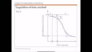
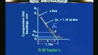
The Log-time curve fitting method is a graphical technique used to estimate the coefficient of consolidation (Cv) of soils based on laboratory data. The essence of this method lies in comparing the theoretical consolidation curve (Uz) with the experimental data plotted on a logarithmic time scale (log Tv).
Steps for Application:
- Plot Dial Readings: Begin by plotting the dial reading of compression for a specific pressure increment against time on a logarithmic scale.
- Select Points: Identify two points (P and Q) on the upper portion of the consolidation curve at times t1 and t2, where t2 is four times t1 (t2 = 4t1).
- Calculate Difference: Define x as the difference in dial readings between points P and Q. Point R is then placed vertically above point P at a distance equal to x.
- Horizontal Line: Draw a horizontal line from R, and the corresponding dial reading at this line is d0, indicating 0% consolidation.
- Project Lines: Extend the primary and secondary consolidation curves to find the intersection point T. The dial reading at T corresponds to d100, signifying 100% consolidation.
This method provides a clear graphical representation of soil behavior under consolidation and aids engineers in predicting settlement and stability issues.
Youtube Videos


Audio Book
Dive deep into the subject with an immersive audiobook experience.
Introduction to the Log-Time Curve Fitting Method
Chapter 1 of 6
🔒 Unlock Audio Chapter
Sign up and enroll to access the full audio experience
Chapter Content
The basis for this method is the theoretical (Uz) versus log Tv curve and experimental dial gauge reading and log t curves are similar.
Detailed Explanation
The log-time curve fitting method is established on the premise that there is a similarity between the theoretical curve (Uz) and the experimental results (log Tv). This means that, when graphs of theoretical values and experimental readings are plotted on a logarithmic scale, they exhibit similar shapes or trends. This method helps in understanding how soil compresses over time under specific conditions.
Examples & Analogies
Think of a gardener who tracks the growth of a plant over time. By plotting the growth on a graph, both the gardener and scientists can observe patterns, just like the similarities observed in theoretical versus experimental curves in soil mechanics.
Step 1: Plotting the Dial Reading
Chapter 2 of 6
🔒 Unlock Audio Chapter
Sign up and enroll to access the full audio experience
Chapter Content
Plot the dial reading of compression for a given pressure increment versus time to log scale.
Detailed Explanation
In the first step, you need to collect data from the compression of soil samples under a specific pressure. This involves measuring how much the soil compresses over time as it is subjected to this pressure. You then plot these readings on a graph using a logarithmic scale for time. The logarithmic scale helps in visualizing changes that might otherwise be hard to see on a linear scale, particularly exponential changes.
Examples & Analogies
Imagine timing how long it takes a sponge to absorb water. By measuring the sponge's size at different intervals (like 1 minute, 2 minutes), you can see how quickly it absorbs water over time. If you plot these absorbent times on a log scale, you can more easily see patterns in the sponge's behavior.
Step 2: Selecting Points on the Curve
Chapter 3 of 6
🔒 Unlock Audio Chapter
Sign up and enroll to access the full audio experience
Chapter Content
Plot two points P and Q on the upper portion of the consolidation curve (say compression line) corresponding to time t1 and t2 such that t2=4t1.
Detailed Explanation
Next, select two specific points on your plotted curve, labeled P and Q. The time associated with point Q should be four times that of point P (i.e., if t1 is 1 minute, then t2 is 4 minutes). This step is crucial because it allows you to examine how the soil behaves as it consolidates over a time span that varies significantly, which reinforces the understanding of the consolidation phenomenon in soil mechanics.
Examples & Analogies
Think of a race where you time two participants covering a distance. If the first participant finishes in 1 minute, and the second in 4 minutes, comparing their performances can reveal insights into how speed changes over time under different conditions.
Step 3: Difference in Dial Readings
Chapter 4 of 6
🔒 Unlock Audio Chapter
Sign up and enroll to access the full audio experience
Chapter Content
Let x be the difference in dial reading between P and Q. Locate R at a vertical distance x above point P.
Detailed Explanation
Here, you quantify the difference in dial readings between the two points P and Q. This difference, labeled as x, represents the change in soil consolidation between the two time points. You then plot an additional point, R, directly above point P on the graph at a vertical distance corresponding to this difference x. This visual representation helps in understanding the consolidation progress visually.
Examples & Analogies
Picture a balloon being inflated. If you measure how much the balloon expands after 1 minute versus 4 minutes, the difference in size correlates to how much air has been added. By marking this difference on your graph, it’s like showing how much ‘growth’ has occurred in your balloon during that time span.
Step 4: Drawing the Horizontal Line
Chapter 5 of 6
🔒 Unlock Audio Chapter
Sign up and enroll to access the full audio experience
Chapter Content
Draw a horizontal line RS; the dial reading corresponding to this line is d0 which corresponds with 0% consolidation.
Detailed Explanation
Once point R is determined, draw a horizontal line to the right. The point where this line intersects the vertical axis of your chart indicates the dial reading at the starting point of consolidation, labeled as d0. This reading effectively serves as a reference point, representing the initial state of the soil before any consolidation has occurred.
Examples & Analogies
Consider using a measuring cup filled with flour. Initially, the flour is piled high, representing your starting point (0% consolidation). Drawing a line across when the flour settles slightly helps you visually gauge how much it has changed after being disturbed.
Step 5: Projecting the Straight Line
Chapter 6 of 6
🔒 Unlock Audio Chapter
Sign up and enroll to access the full audio experience
Chapter Content
Project the straight line portion of primary and secondary consolidation to intersect at point T. The dial reading corresponding to T is d100 and this corresponds to 100% consolidation.
Detailed Explanation
Finally, extend the segments of your graph that represent primary and secondary consolidation until they meet at a new point T. The reading at this intersection represents d100, which indicates that the soil has fully consolidated (100%). This step is critical because it helps in predicting the final behavior of the soil under prolonged pressure, providing essential data for engineering decisions.
Examples & Analogies
Think of a sponge fully soaked in water. As you continue to submerge it, water will stop being absorbed once it's fully saturated. The final state of saturation represents the point where no more water can enter, similar to the concept of 100% consolidation in soils.
Key Concepts
-
Log-Time Curve: A graphical representation that helps analyze soil consolidation data.
-
Dial Gauge: An instrument used to measure the extent of compression in soils during consolidation testing.
-
Consolidation Curve: A plot representing the relationship between the degree of consolidation and time.
Examples & Applications
An engineering project involves measuring how much a building's foundation settles over time using the log-time curve fitting method.
Graphs of consolidation data using different methods highlight the contrast in results obtained through the log-time curve fitting method.
Memory Aids
Interactive tools to help you remember key concepts
Rhymes
In the Log-time method, don’t you see, we plot it quick and easily!
Stories
Imagine a tiny building on soft soil. As time passes, it slowly sinks. You plot this process like a race to see how fast it settles, using the Log-time method to help visualize the journey.
Memory Tools
Remember 'PQR'—Plot, Query, Read to consolidate smoothly in the Log-time method.
Acronyms
LTC (Log-Time Curve) helps engineers calculate consolidation effortlessly!
Flash Cards
Glossary
- Coefficient of Consolidation (Cv)
A measure of the rate at which soil consolidates when subjected to a load.
- Dial Reading
The measurement taken from the dial gauge to assess the compression of soil.
- Log Scale
A scale used to plot data where each unit increase represents an exponential increase in value.
- Primary Consolidation
The initial stage of the consolidation process which involves a decrease in volume due to pore water expulsion.
- Secondary Consolidation
The stage following primary consolidation, where additional settlement occurs due to the rearrangement of soil particles.
Reference links
Supplementary resources to enhance your learning experience.