
Square root of time method
Enroll to start learning
You’ve not yet enrolled in this course. Please enroll for free to listen to audio lessons, classroom podcasts and take practice test.
Interactive Audio Lesson
Listen to a student-teacher conversation explaining the topic in a relatable way.
Introduction to Square root of time method
🔒 Unlock Audio Lesson
Sign up and enroll to listen to this audio lesson

Today, we will discuss the Square root of time method. Can anyone tell me the significance of this method in consolidation testing?

Is it used to calculate how quickly soil consolidates under pressure?
Exactly! This method is a graphical technique that helps us estimate the coefficient of consolidation, or Cv, based on time and dial readings.

How do we start implementing this method?
We begin by plotting dial readings against time using a log scale. Remember, the relationship we establish here is crucial for understanding how soil behaves over time.

What does it mean for time points to be in a certain ratio?
Great question! We typically select two points where the time at the second point is four times that of the first, which is key in our calculations.

How do we find those points on the graph?
You will look for points on the upper part of the consolidation curve, then calculate the difference in dial readings to find additional points like R.
To summarize, starting with a plot of dial readings on a log scale, identifying specific time ratios, and plotting those accurately is essential for this method.
Executing the Square root of time Method
🔒 Unlock Audio Lesson
Sign up and enroll to listen to this audio lesson

Now that we have the basics down, let's elaborate on the steps to effectively execute the Square root of time method.
How do we find the two points, P and Q, for our calculations?
You need to identify those points where time is precisely in a 1:4 ratio. The gap in dial readings between these points will pave the way for our calculations.
What do we do after identifying these points?
After plotting points P and Q, we locate point R by measuring the vertical distance, which helps us determine the initial consolidation reading, d0.
And what about reaching 100% consolidation?
To find 100% consolidation, project the lines until they meet to create point T, which helps us establish d100, giving us the maximum consolidation reading.
In summary, engaging with these concepts through plotting and projection illustrates the consolidation process visually and mathematically.
Practical Considerations and Conclusion
🔒 Unlock Audio Lesson
Sign up and enroll to listen to this audio lesson
As we conclude, can anyone summarize the benefits of using the Square root of time method?
It provides a clear graphical representation of consolidation over time and helps identify key consolidation markers.
Absolutely! It not only aids in determining Cv but enhances our insight into soil behavior.
Is this method suitable for all types of soil?
Good point—while it's broadly applicable, the nature of the soil can influence how effective this method is.
How can we ensure accuracy in our measurements and plots?
Using precise instruments and ensuring correct scaling on our plots is vital for accurate interpretation of the results.
To wrap up, the Square root of time method is a valuable tool in geotechnical engineering that exemplifies the practical application of theory to real-world issues in soil testing.
Introduction & Overview
Read summaries of the section's main ideas at different levels of detail.
Quick Overview
Standard
This section discusses the Square root of time method as part of the process for estimating the coefficient of consolidation (Cv) using graphical techniques. Key steps for constructing the necessary plots are highlighted to facilitate understanding of how time affects consolidation.
Detailed
Square Root of Time Method
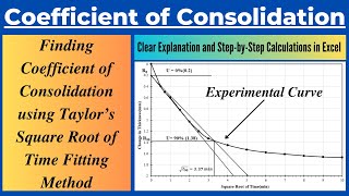
The Square root of time method is an essential graphical technique utilized in soil mechanics to determine the coefficient of consolidation (Cv) from laboratory consolidation tests. This method, along with others like the logarithm of time method and hyperbola method, provides a visual approach to understand how consolidation occurs over time. In this section, the primary steps involved in applying the Square root of time method are outlined, emphasizing how to generate and interpret the relevant plots:
- Initial Setup: Begin by preparing your data from the consolidation test and plot the dial gauge readings against time on a log scale.
- Identification of Points: Identify two specific points (P and Q) on the consolidation curve where the time at point Q is four times the time at point P (i.e., t2 = 4t1).
- Dial Reading Difference: Calculate the difference in dial readings between points P and Q, denoted as x. Use this value to establish another point, R, which is positioned a vertical distance of x above point P.
- Set d0 and d100: From point R, draw a horizontal line to identify the dial reading, d0, which corresponds to 0% consolidation. Continue projecting the straight line portions of primary and secondary consolidation until they intersect at point T. The reading at point T indicates 100% consolidation and is denoted as d100.
Through these steps, the Square root of time method encapsulates how the consolidation process is quantified over time and illuminates the relationship between dial gauge readings and consolidation percentages.
Youtube Videos


Audio Book
Dive deep into the subject with an immersive audiobook experience.
Introduction to the Square Root of Time Method
Chapter 1 of 3
🔒 Unlock Audio Chapter
Sign up and enroll to access the full audio experience
Chapter Content
The coefficient of three graphical procedure are used:
1. Logarithm of time method
2. Square root of time method
3. Hyperbola method
Detailed Explanation
The square root of time method is one of three techniques used to determine the coefficient of consolidation (Cv) from laboratory data. This method, along with the logarithm of time method and the hyperbola method, provides different frameworks for analyzing soil consolidation behavior. The square root of time method focuses on the relationship between consolidation time and the amount of consolidation that occurs, leveraging the mathematical property that consolidation rate is proportional to the square root of time.
Examples & Analogies
Imagine you are planting a small tree in your backyard and want to understand how quickly the soil settles around it. You can observe that as time passes, the soil compresses around the roots. Just like with soil consolidation, the more time passes, the more tightly the soil will settle. In the square root of time method, we essentially quantify this 'settling process' so that we can predict how long it will take for the soil to fully consolidate around the tree.
Steps for the Square Root of Time Method
Chapter 2 of 3
🔒 Unlock Audio Chapter
Sign up and enroll to access the full audio experience
Chapter Content
Log – time curve fitting method:
1. Plot the dial reading of compression for a given pressure increment versus time to log scale.
2. Plot two points P and Q on the upper portion of the consolidation curve (say compression line) corresponding to time t1 and t2 such that t2=4t1.
3. Let x be the difference in dial reading between P and Q. locate R at a vertical distance x above point P.
4. Draw a horizontal line RS the dial reading corresponding to this line is d0 which corresponds with 0% consolidation.
Detailed Explanation
The steps of the square root of time method involve plotting data from a soil compression test. First, you collect data on how much the soil compresses under a specific amount of pressure and plot this data against time on a logarithmic scale. Then, select two specific timestamps (t1 and t2) related by the formula t2 = 4t1. Next, calculate the change in dial readings (x) between these time points and mark it on the graph to visualize the current state of consolidation. The horizontal line drawn at this step represents the degree of consolidation up to that point, labeled as d0.
Examples & Analogies
Think of setting up dominoes in a line. When you push the first domino, they start to fall one by one. If you time how long it takes for the first half of the dominoes to fall (t1) and then observe the second half (t2 = 4t1), you can see how the total effect increases over time. In the experiment, you plot these times and the changes in height like you would plot which dominoes have fallen and their corresponding times.
Completing the Plot
Chapter 3 of 3
🔒 Unlock Audio Chapter
Sign up and enroll to access the full audio experience
Chapter Content
- Project the straight line portion of primary and secondary consolidation to intersect at point T. The dial reading corresponding to T is d100 and this corresponds to 100% consolidation.
Detailed Explanation
In the final step, you will extrapolate the data plotted to visualize the overall trend of consolidation. This involves projecting the plotted line segments from the initial points towards where they would theoretically intersect if continued, ending at point T. The reading at this new point (d100) reflects that the soil has fully consolidated and can be interpreted as reaching 100% consolidation.
Examples & Analogies
Imagine you’re tracking how far a car travels over time. You start measuring distance at various points and notice that at some point, you slow down just before hitting the maximum speed. By extending your observations on a graph, you can predict when you would reach your top speed, similar to predicting the total consolidation of soil using extrapolated points in the graph.
Key Concepts
-
Coefficient of Consolidation (Cv): This is a critical parameter in soil mechanics that quantifies the soil's rate of consolidation under loading over time.
-
Logarithmic Plotting: Using a log scale to represent time allows for clarity in visualizing rapid changes over extended periods.
-
Dial Gauge Measurement: The readings taken from a dial gauge help in determining the extent of soil compression directly correlating to consolidation.
Examples & Applications
An example of using the Square root of time method is applying it to determine Cv from laboratory retraction measurements after applying a uniform load on a soil sample.
Another instance would be plotting a consolidation test result where points P and Q represent different elapsed times for soil under test, allowing engineers to visualize the relationship between time and consolidation.
Memory Aids
Interactive tools to help you remember key concepts
Rhymes
For soil that sits and waits, time determines its fates; with points P and Q in sight, consolidation feels just right.
Stories
Imagine a farmer testing land. He uses different tools — a dial gauge here and a graph paper there. Over time, he watches how the soil compresses under weight, finding that when he plots certain points, he can forecast the soil's future.
Memory Tools
DPR - Dial, Points, Ratio. Remember this sequence to recall key elements in the Square root of time method.
Acronyms
Cv - Consolidation Velocity. Use this acronym to remember the goal of the method, which is determining how fast soils can consolidate.
Flash Cards
Glossary
- Coefficient of Consolidation (Cv)
A parameter that quantifies the rate at which a soil material consolidates under loading.
- Consolidation Curve
A graph representing the relationship between time and deformation of a soil under stress.
- Log Scale
A nonlinear scale used to represent large ranges of values, often used in time plotting.
Reference links
Supplementary resources to enhance your learning experience.