
Infiltration Equations and Models
Enroll to start learning
You’ve not yet enrolled in this course. Please enroll for free to listen to audio lessons, classroom podcasts and take practice test.
Interactive Audio Lesson
Listen to a student-teacher conversation explaining the topic in a relatable way.
Horton’s Equation
🔒 Unlock Audio Lesson
Sign up and enroll to listen to this audio lesson

Today, we start with Horton’s Equation, which describes how the infiltration rate changes over time. Can anyone tell me what infiltration means?

Isn’t it how water enters the soil?
Exactly! Now, Horton’s Equation can be expressed as f(t) = f0 + (fc - f0)e^(-kt). Here, f(t) represents the infiltration rate at time t. Why do you think the infiltration rate decreases as time goes on?

Maybe because the soil gets saturated?
Great observation! The initial infiltration rate is generally high, but it declines as the soil becomes saturated. This brings us to the importance of understanding the decay constant, k. What do you think it signifies?

Could it determine how quickly the rate decreases?
Correct! The decay constant is essential for modeling how quickly the infiltration process slows down. So, in short, Horton’s model effectively captures the declining infiltration rate over time.
Philip’s Equation
🔒 Unlock Audio Lesson
Sign up and enroll to listen to this audio lesson

Moving on, let’s talk about Philip’s Equation, which accounts for capillarity and gravity in water movement. The equation is f(t) = St^(-1/2) + A. Can anyone explain what 'sorptivity' means in this context?
Isn’t it related to how well water can be absorbed by the soil?
Exactly! Sorptivity indicates how quickly the soil can absorb water. This equation is particularly useful for short-duration infiltration events. Why do we think that might be?
Because it describes quick saturation events?
Spot on! It helps us analyze conditions like rainfall. Philip's equation complements Horton's by focusing on capillary action and gravity effects. So, we now have a broader understanding of how water infiltrates the soil.
Green-Ampt Equation
🔒 Unlock Audio Lesson
Sign up and enroll to listen to this audio lesson
Let’s now explore the Green-Ampt Equation. This model applies when we assume a sharp wetting front, especially under ponded conditions. The formula is f = K(1 + ψ(θs - θi))F. What do you think each term represents?
I think K is hydraulic conductivity?
Correct! Hydraulic conductivity indicates how fast water can flow through the soil. Now, what about the term 'wetting front suction head'?

Does it have to do with the pressure at the front of the water moving in?
Exactly! It helps determine how easily water can move into drier soil. The cumulative infiltration F is also critical as it shows how much water has moved in over time. Why do we consider this equation particularly accurate?
Because it works well for homogeneous soils?
Right again! Understanding the Green-Ampt model enriches our comprehension of infiltration in specific conditions and improves predictions.
Introduction & Overview
Read summaries of the section's main ideas at different levels of detail.
Quick Overview
Standard
In this section, we explore the mathematical models that describe infiltration behavior over time. Horton’s Equation, Philip’s Equation, and Green-Ampt Equation are essential for understanding infiltration dynamics, each offering unique insights and applications in hydrology and engineering.
Detailed
Infiltration Equations and Models
Infiltration equations and models play a critical role in quantifying how water moves from the soil surface into the profile. Understanding these models is essential due to the implications for hydrology, irrigation design, and water resource management.
1. Horton’s Equation
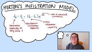
- Overview: Developed by Robert E. Horton, this equation models the infiltration rate over time. It indicates that infiltration starts high and declines exponentially until it stabilizes at a lower rate.
- Formula:
f(t) = f0 + (fc - f0)e^(-kt)where: f(t): infiltration rate at time tf0: initial infiltration ratefc: final infiltration ratek: decay constantt: time
2. Philip’s Equation
- Overview: This equation relates infiltration to capillary and gravity forces, useful for analyzing short-duration rainfall.
- Formula:
f(t) = St^(-1/2) + Awhere: S: sorptivityA: steady infiltration rate due to gravity
3. Green-Ampt Equation
- Overview: A physically-based model assuming a sharp wetting front, applied primarily in ponded conditions, offers high accuracy for homogeneous soils.
- Formula:
f = K(1 + ψ(θs - θi))Fwhere: K: hydraulic conductivityψ: wetting front suction headθs: saturated moisture contentθi: initial moisture contentF: cumulative infiltration
Understanding these equations provides engineers with vital tools for estimating infiltration rates, which is crucial for effective water management and irrigation system designs.
Youtube Videos


Audio Book
Dive deep into the subject with an immersive audiobook experience.
Horton’s Equation
Chapter 1 of 3
🔒 Unlock Audio Chapter
Sign up and enroll to access the full audio experience
Chapter Content
Developed by Robert E. Horton:
f(t)=f_0 + (f_c - f_0)e^{-kt}
Where:
- f(t): infiltration rate at time t
- f_0: initial infiltration rate
- f_c: final/constant infiltration rate
- k: decay constant
- t: time
Horton’s model fits well with field data and represents the declining infiltration rate over time.
Detailed Explanation
Horton’s Equation is a mathematical formula used to describe how the rate of infiltration changes over time. Initially, when water begins infiltrating the soil, the rate is high, often represented by f_0. As time passes, environmental conditions such as soil saturation cause this rate to decrease, approaching a final steady value, f_c. The decay constant, k, determines how quickly this decrease occurs. By using this equation, engineers can predict how quickly and efficiently water will infiltrate into various soil types, which is crucial for water management.
Examples & Analogies
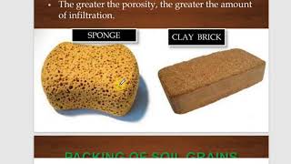
Think of Horton’s equation like a sponge soaking up water. When you first pour water on a dry sponge (initial infiltration), it absorbs rapidly. But as the sponge becomes wetter, it absorbs more slowly until it can hold no more water (steady infiltration). This equation helps engineers understand how quickly and how much water will enter the ground compared to that initial rapid absorption.
Philip’s Equation
Chapter 2 of 3
🔒 Unlock Audio Chapter
Sign up and enroll to access the full audio experience
Chapter Content
Based on capillarity and gravity forces:
f(t) = S t^{-1/2} + A
Where:
- S: sorptivity (depends on soil suction and porosity)
- A: steady infiltration rate due to gravity
It is useful for short-duration infiltration analysis.
Detailed Explanation
Philip’s Equation accounts for both the capillary action of the soil and the gravitational forces acting on water. The term 'S' reflects how quickly water can enter the soil based on its properties, while 'A' represents a constant rate of infiltration due to gravity once the soil is saturated. This equation is particularly useful for analyzing how much water will infiltrate during short rain events, allowing engineers to estimate immediate soil absorption rates effectively.
Examples & Analogies
Imagine trying to pour syrup on a stack of pancakes. At the start, the syrup can soak in quickly due to the light, fluffy pancake texture (sorptivity), but as you continue to pour (increased saturation), it starts to flow off (steady rate). Philip’s equation helps predict how this process works for soil and water.
Green-Ampt Equation
Chapter 3 of 3
🔒 Unlock Audio Chapter
Sign up and enroll to access the full audio experience
Chapter Content
A physically based model assuming a sharp wetting front:
f = K rac{ ext{ψ}( heta_s - heta_i)}{F}
Where:
- K: hydraulic conductivity
- ψ: wetting front suction head
- θ_s: saturated moisture content
- θ_i: initial moisture content
- F: cumulative infiltration
Detailed Explanation
The Green-Ampt Equation models infiltration by considering how a wetting front moves through the soil. The hydraulic conductivity (K) measures how easily water can flow through the soil, while the wetting front suction head (ψ) indicates how deeply the water is penetrating. This equation provides a more comprehensive understanding of water movement in soil, taking both initial moisture content and total infiltrated water into account. It is particularly accurate for scenarios where there is a clear transition from dry to wet soil, known as a wetting front.
Examples & Analogies
Consider when you water a dry lawn. Initially, the water quickly saturates the top layer (the wetting front), pushing down through the soil. The Green-Ampt Equation helps predict how fast and deep that water will travel, similar to the way a wave moves through sand at the beach, creating layers of wet and dry sand.
Key Concepts
-
Horton’s Equation: A model describing the decline of the infiltration rate over time.
-
Philip’s Equation: An equation that integrates capillary and gravity influences on infiltration.
-
Green-Ampt Equation: A physically based model for infiltration, particularly effective under ponded conditions.
Examples & Applications
Using Horton’s Equation, an engineer estimates the infiltration rate for a specific rainfall event to determine runoff potential.
Philip’s Equation can help analyze the infiltration for short-duration storms, providing critical insights for irrigation planning.
Applying the Green-Ampt Equation allows for accurate predictions of how much water will infiltrate during a flood event in agricultural settings.
Memory Aids
Interactive tools to help you remember key concepts
Rhymes
Horton's Equation works just fine, its rates decline over time!
Stories
Imagine a farmer observing the pouring rain, their fields soak quickly at first, then slow down. This depicts Horton’s model perfectly!
Memory Tools
PSG for remembering the models: P for Philip, S for Sorptivity, G for Green-Ampt.
Acronyms
HGL for Horton, Green-Ampt, and Leaf - capturing key models of infiltration.
Flash Cards
Glossary
- Horton’s Equation
An empirical equation that models the infiltration rate over time, showing a decrease as the soil becomes saturated.
- Sorptivity
A measure of the soil's capacity to absorb water, influenced by capillary forces.
- Hydraulic Conductivity
The property of soil that describes its ability to transmit water through its pores.
- Cumulative Infiltration
The total amount of water that has infiltrated into the soil over a specified period.
Reference links
Supplementary resources to enhance your learning experience.