
Key Differences Between Ideal and Real Op-Amps
Interactive Audio Lesson
Listen to a student-teacher conversation explaining the topic in a relatable way.
Open-Loop Gain
🔒 Unlock Audio Lesson
Sign up and enroll to listen to this audio lesson

Today, we're going to discuss the open-loop gain of op-amps. Can anyone tell me what this means?

Is it how much the op-amp can amplify a signal without any feedback?
Exactly! For an ideal op-amp, the gain is infinite, which means even the smallest difference will result in a huge output. But what about real op-amps?

I think real op-amps have a finite gain, like 10,000 to 1,000,000.
Correct! This limitation means they might not respond linearly to small input differences. Remember the acronym FIO: 'Finite Input Output'.

What happens if we use feedback then?
Great question, Student_3! Using feedback helps control the gain and improve stability. Let's summarize: ideal op-amps have infinite gain, while real op-amps have finite gain.
Input and Output Impedance
🔒 Unlock Audio Lesson
Sign up and enroll to listen to this audio lesson

Next, let's explore input and output impedance. Does anyone know the significance of these parameters?

Input impedance is really high for ideal op-amps, right?
Exactly! Ideal op-amps have infinite input impedance, meaning they don’t draw current from the source. However, what about real op-amps?
They have high but finite input impedance, which can affect signal integrity.
Exactly! Now, output impedance is different. Ideal op-amps have zero output impedance. What does that mean for real op-amps?
It means they can’t drive loads as effectively as ideal ones?
Great job! This leads to possible voltage drops when driving heavy loads. So, what can we conclude about impedance?
Real op-amps have finite input and non-zero output impedances, affecting performance.
Well summarized! Always remember the role of impedance in designing circuits.
Bandwidth and Noise
🔒 Unlock Audio Lesson
Sign up and enroll to listen to this audio lesson
Now let’s talk about bandwidth. What does infinite bandwidth mean for an ideal op-amp?
It means it can amplify any frequency signal without limitations!
Correct! In contrast, real op-amps have limited bandwidth. What does this imply for circuit designers?
They need to consider the Gain-Bandwidth Product, right?
Exactly! The product of gain and bandwidth helps determine the frequency response. Now, let’s tie it in with noise. What do we know?
Real op-amps introduce noise due to internal components.
Yes! This noise can affect precision applications. So, what should be our takeaway about bandwidth and noise?
Both affect signal quality and must be considered in design.
Excellent! That’s the essence of using op-amps practically.
Introduction & Overview
Read summaries of the section's main ideas at different levels of detail.
Quick Overview
Standard
In this section, we compare the idealized characteristics of operational amplifiers (op-amps) to their real-world counterparts, highlighting key parameters where they differ. Real op-amps exhibit finite open-loop gain, limited bandwidth, and non-zero output impedance, which affect their application in various electronic circuits.
Detailed
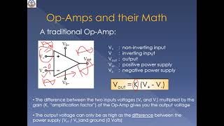
Key Differences Between Ideal and Real Op-Amps
This section delineates the fundamental contrasts between ideal and real operational amplifiers (op-amps). While ideal op-amps are theoretical constructs with perfect characteristics, real op-amps operate under various physical limitations that impact their performance. Below are the critical differences:
Characteristics Comparison
| Characteristic | Ideal Op-Amp | Real Op-Amp |
|---|---|---|
| Open-Loop Gain (Aₒ) | Infinite | Finite (10⁴ to 10⁶) |
| Input Impedance | Infinite | High, but finite (MΩ range) |
| Output Impedance | Zero | Non-zero, typically low |
| Bandwidth | Infinite | Limited, with Gain-Bandwidth Product |
| Offset Voltage | Zero | Non-zero (typically mV) |
| Input Bias Current | Zero | Small current (nA to μA) |
| Noise | Zero | Present due to internal components |
| Power Supply Requirement | Idealized (no limits) | Requires dual power supply (positive and negative) |
| Slew Rate | Infinite | Finite (limited by design) |
These differences have significant implications on the design and analysis of practical circuits, emphasizing the importance of considering the characteristics of real op-amps in engineering applications.
Youtube Videos


Audio Book
Dive deep into the subject with an immersive audiobook experience.
Open-Loop Gain Differences
Chapter 1 of 9
🔒 Unlock Audio Chapter
Sign up and enroll to access the full audio experience
Chapter Content
Characteristic Ideal Op-Amp Real Op-Amp
Open-Loop Gain (Aₒ) Infinite Finite (10⁴ to 10⁶)
Detailed Explanation
The open-loop gain of an ideal op-amp is assumed to be infinite, meaning any tiny difference between the input voltages results in a maximal output. In contrast, real op-amps have a finite open-loop gain, which typically ranges from 10,000 to 1,000,000. This limitation implies that real op-amps do not respond perfectly to small input changes, especially without feedback. As a result, their accuracy in amplifying a signal can be less than ideal.
Examples & Analogies
Think of a microphone that can amplify sound perfectly without distortion as an ideal op-amp. However, in reality, microphones may not be able to pick up the quietest sounds perfectly due to limitations in their components, much like a real op-amp's finite gain.
Input Impedance Differences
Chapter 2 of 9
🔒 Unlock Audio Chapter
Sign up and enroll to access the full audio experience
Chapter Content
Characteristic Ideal Op-Amp Real Op-Amp
Input Impedance Infinite High, but finite (MΩ range)
Detailed Explanation
An ideal op-amp has infinite input impedance, which means it does not draw any current from the input source, ensuring that the source signal remains undisturbed. However, real op-amps have a high but finite input impedance, typically in the megaohm range. This means a small amount of current is drawn, which can affect the integrity of the input signal, especially in sensitive applications such as sensor readings where high accuracy is needed.
Examples & Analogies
Imagine a sponge soaking up water; an ideal op-amp would be a perfect sponge that doesn’t absorb a drop of water, while a real op-amp is like a sponge that absorbs just a little water. If there's too much absorption, it will leave less water for other uses, similar to how a real op-amp can affect the input signal.
Output Impedance Differences
Chapter 3 of 9
🔒 Unlock Audio Chapter
Sign up and enroll to access the full audio experience
Chapter Content
Characteristic Ideal Op-Amp Real Op-Amp
Output Impedance Zero Non-zero, typically low
Detailed Explanation
Ideal op-amps are assumed to have zero output impedance, which means they can deliver any amount of current without losing voltage across their output terminals. In contrast, real op-amps have some non-zero output impedance, though it is low. This can affect the op-amp's ability to drive loads, particularly when the load resistance is low, potentially causing voltage drops.
Examples & Analogies
Think of a water hose (ideal op-amp): it can deliver water without any back pressure (zero output impedance). A real hose, however, has some resistance (non-zero output impedance) that might reduce the flow if a heavy object were to be pushed against the water, illustrating how real op-amps can struggle under certain loads.
Bandwidth Differences
Chapter 4 of 9
🔒 Unlock Audio Chapter
Sign up and enroll to access the full audio experience
Chapter Content
Characteristic Ideal Op-Amp Real Op-Amp
Bandwidth Infinite Limited, with Gain-Bandwidth Product
Detailed Explanation
An ideal op-amp is assumed to have infinite bandwidth, allowing it to amplify signals of all frequencies without any loss. However, real op-amps have a limited bandwidth and their performance varies with frequency due to what’s known as the Gain-Bandwidth Product (GBW)—a constant for a given op-amp that describes how gain decreases as bandwidth increases.
Examples & Analogies
Consider an athlete running at a sprint: an ideal athlete can maintain an incredible speed indefinitely without tiring. In contrast, a real athlete can sprint fast for a short time but will eventually slow down due to fatigue. Similarly, real op-amps can only maintain high gain at lower frequencies before their performance drops off.
Offset Voltage Differences
Chapter 5 of 9
🔒 Unlock Audio Chapter
Sign up and enroll to access the full audio experience
Chapter Content
Characteristic Ideal Op-Amp Real Op-Amp
Offset Voltage Zero Non-zero (typically mV)
Detailed Explanation
In ideal op-amps, there is no offset voltage, meaning both inputs are perfectly balanced when the output is zero. However, real op-amps have a non-zero offset voltage, which can vary typically in the millivolt range, leading to discrepancies in output even when no signal is present. This offset can introduce notable errors in sensitive applications requiring precision.
Examples & Analogies
Imagine trying to balance a seesaw perfectly: an ideal seesaw remains level without any effort. A real seesaw, however, might lean to one side slightly due to uneven weight distribution (offset voltage), leading to issues or wrong readings in applications like weighing scales.
Input Bias Current Differences
Chapter 6 of 9
🔒 Unlock Audio Chapter
Sign up and enroll to access the full audio experience
Chapter Content
Characteristic Ideal Op-Amp Real Op-Amp
Input Bias Current Zero Small current (nA to μA)
Detailed Explanation
An ideal op-amp introduces no input bias current, meaning that no current flows into the input terminals. In contrast, real op-amps do draw a small amount of input bias current, typically in the nanoamp to microamp range. This current can lead to voltage drops across components connected to the input, causing signal inaccuracies, especially in high-impedance circuits.
Examples & Analogies
Consider an empty glass (ideal op-amp) that doesn’t leak any liquid; you could pour as much as you want without worry. Now, imagine a glass with a small crack (real op-amp) that lets a tiny bit of liquid escape over time; this continuous loss can result in inaccurate measurements, much like input bias can distort signals in high-impedance scenarios.
Noise Differences
Chapter 7 of 9
🔒 Unlock Audio Chapter
Sign up and enroll to access the full audio experience
Chapter Content
Characteristic Ideal Op-Amp Real Op-Amp
Noise Zero Present due to internal components
Detailed Explanation
Ideal op-amps are noise-free, meaning they do not add any unwanted signals to the system. Real op-amps, however, introduce noise due to internal components like transistors and resistors. This noise can affect high-precision applications and is especially significant in circuits that operate at high frequencies, where the noise can interfere with the intended signals.
Examples & Analogies
Think of a perfectly quiet library (ideal op-amp) where no sound disrupts your reading. A real library may have soft background noises (real op-amp noise) like pages turning or distant conversations, which can distract you, just as noise in op-amps can interfere with signal clarity in sensitive applications.
Power Supply Differences
Chapter 8 of 9
🔒 Unlock Audio Chapter
Sign up and enroll to access the full audio experience
Chapter Content
Characteristic Ideal Op-Amp Real Op-Amp
Power Supply Idealized (no limits) Requires dual power supply (positive and negative)
Detailed Explanation
The ideal op-amp can be powered without any limitations, implying that it could function perfectly under any power supply condition. On the other hand, real op-amps generally require a dual power supply, which means both positive and negative voltages are often needed to operate optimally. This power supply configuration is essential to ensure the proper functioning of the circuit and to handle both positive and negative signal swings.
Examples & Analogies
Imagine a car (ideal op-amp) that can run indefinitely without refueling. A real car needs specific types of fuel (real op-amp requirements) — like gasoline and diesel — depending on its design, illustrating that practical tools have specific energy needs.
Slew Rate Differences
Chapter 9 of 9
🔒 Unlock Audio Chapter
Sign up and enroll to access the full audio experience
Chapter Content
Characteristic Ideal Op-Amp Real Op-Amp
Slew Rate Infinite Finite (limited by design)
Detailed Explanation
The slew rate of an ideal op-amp is considered infinite, implying it can change its output instantaneously in response to input signal changes. In real op-amps, the slew rate is finite, which means there are limits to how quickly the output can respond. This limitation can affect the response to fast-changing signals, especially in high-frequency applications.
Examples & Analogies
Think of a professional sprinter (ideal op-amp) who can instantly change speeds in a race. A regular person (real op-amp), however, may take a moment to reach top speed. This time lag can affect the outcome, similar to how real op-amps can lag in response to rapid input changes, impacting their performance in fast electronics.
Key Concepts
-
Open-Loop Gain: The output/input voltage ratio of an op-amp without feedback, ideally infinite for ideal op-amps.
-
Input Impedance: The resistance the op-amp presents at its input; ideal is infinite to prevent drawing current.
-
Output Impedance: The resistance at the output of the op-amp; ideally zero for effective load driving.
-
Bandwidth: The frequency range within which the op-amp operates effectively; ideal is infinite, but real op-amps are limited.
-
Noise: Random electrical signals from internal components of op-amps affecting precision.
Examples & Applications
An ideal op-amp can amplify a 1mV input to 10V without feedback due to infinite gain, while a real op-amp with a gain of 100,000 may produce significantly less output depending on the inputs.
In an audio circuit, using a real op-amp, even small noise levels present may distort the sound, while an ideal op-amp would produce a perfectly clear signal.
Memory Aids
Interactive tools to help you remember key concepts
Rhymes
In an op-amp world so bright and wide, infinite gain is the ideal guide.
Stories
Imagine a perfect op-amp at a party—it never tires and amplifies every whisper, while its real-world cousin sometimes struggles to hear over the noise.
Memory Tools
Gains And Impedances Must Be Quiet — Remember this for understanding Gain, Input, and Output impedances, Noise in op-amps.
Acronyms
GIB NO (Gain, Input, Bandwidth, Noise, Output) — It’s what real op-amps lack compared to ideal ones.
Flash Cards
Glossary
- OpenLoop Gain
The ratio of the output voltage to the input voltage for an op-amp when no feedback is applied, ideally infinite in ideal op-amps.
- Input Impedance
The impedance presented by the input terminals of an op-amp, ideally infinite to avoid drawing current.
- Output Impedance
The impedance presented at the output terminals of an op-amp; ideally zero to drive loads effectively.
- Bandwidth
The range of frequencies over which an op-amp can operate effectively; ideally infinite but finite in real op-amps.
- Noise
Unwanted electrical signals or disturbances introduced by the op-amp's internal components.
- Slew Rate
The maximum rate of change of the output voltage of an op-amp in response to a step input; finite in real op-amps.
Reference links
Supplementary resources to enhance your learning experience.