
Solution by Undetermined Coefficients
Enroll to start learning
You’ve not yet enrolled in this course. Please enroll for free to listen to audio lessons, classroom podcasts and take practice test.
Interactive Audio Lesson
Listen to a student-teacher conversation explaining the topic in a relatable way.
Linear Non-Homogeneous Differential Equations
🔒 Unlock Audio Lesson
Sign up and enroll to listen to this audio lesson

Today, we're going to explore linear non-homogeneous differential equations. Can someone tell me what we mean by 'non-homogeneous'?

I think it means that the equation has terms that are not solely dependent on the function we are solving for, like external forces?
Exactly! In these equations, there's a forcing term, represented as f(x). This term drives the system's response. The general equation can be represented as: ay'' + by' + cy = f(x). Knowing this helps us find the solution.

So we find two parts: the complementary function and the particular integral?
Yes! The complementary function, y_c, solves the homogeneous part — that is, when f(x) = 0. The particular integral, y_p, addresses the non-homogeneous part. Remember, together they give us the general solution!
Conditions for Applying the Method
🔒 Unlock Audio Lesson
Sign up and enroll to listen to this audio lesson

Now, let's talk about when we can actually apply the method of undetermined coefficients. What types of functions should f(x) be?

I read that it can be polynomials, exponentials, or sinusoids, right?
Correct! It must be one of these forms. If it’s a natural log or a piecewise function, this method won't work. Can anyone provide an example of a polynomial we might encounter?

How about f(x) = x^2 + 2x + 1? It’s a quadratic polynomial!
Great example! Remember, identifying the correct form of f(x) is crucial for solving the equation effectively.
Steps in the Undetermined Coefficients Method
🔒 Unlock Audio Lesson
Sign up and enroll to listen to this audio lesson
Let's outline the steps in the undetermined coefficients method. What’s our first step?
We need to solve the homogeneous equation and find the complementary function, right?
Exactly! Then, we guess the form of the particular integral based on the type of f(x). What happens next?
We modify the trial solution if it overlaps with the complementary function?
Correct! After modifying, we substitute back into the original equation and solve for the coefficients. Finally, we combine both functions for the general solution.
Illustrative Examples
🔒 Unlock Audio Lesson
Sign up and enroll to listen to this audio lesson
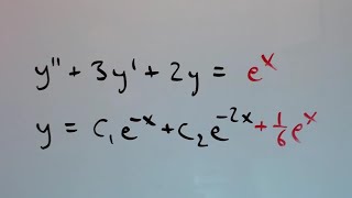
Let's go through some examples to solidify what we've learned. Who would like to solve the equation y'' - 3y' + 2y = e^x?
I can try! First, I find the complementary function. The auxiliary equation is r^2 - 3r + 2 = 0.
Yes, and what are the roots?
The roots are r = 1 and r = 2, so the complementary function is C1e^x + C2e^(2x).
Perfect! Now, what do we do next?
Since e^x is a part of the complementary function, we guess y_p = Axe^x.
Applications in Civil Engineering
🔒 Unlock Audio Lesson
Sign up and enroll to listen to this audio lesson
Lastly, let's talk about how the undetermined coefficients method is applied in civil engineering. Can anyone think of an application?
Beam deflections, I know they can be modeled using this method!
Exactly! Structural analysis often requires solving differential equations that include external loads represented as polynomials or sinusoidal functions. What about mechanical vibrations?
The vibrations of structures! The forcing function can be sinusoidal, making this method very useful!
Great connections! This method is vital in making practical and effective engineering decisions.
Introduction & Overview
Read summaries of the section's main ideas at different levels of detail.
Quick Overview
Standard
The section explains how to apply the method of undetermined coefficients to find particular integrals of non-homogeneous linear differential equations with constant coefficients. It outlines the necessary conditions, key steps involved in the method, and provides illustrative examples.
Detailed
Solution by Undetermined Coefficients
In this section, we explore the method of undetermined coefficients, a crucial technique for solving non-homogeneous linear differential equations with constant coefficients. The general form of these equations is presented, along with their solutions: the complementary function (solution of the homogeneous equation) and the particular integral (solution to the non-homogeneous equation).
Overview
The method is particularly efficient for specific types of non-homogeneous terms, such as polynomials, exponentials, and trigonometric functions. We delve into the necessary conditions for applying this method and outline a systematic procedure to find the particular integral.
Key Steps in the Method
- Solve the Homogeneous Equation: Find the roots of the auxiliary equation to obtain the complementary function.
- Guess the Form of the Particular Integral: Based on the type of forcing function, decide on a trial solution.
- Modify Trial Solution if Needed: Adjust the trial solution if it overlaps with the complementary function.
- Substitute and Determine Coefficients: Substitute the trial solution into the original equation and equate coefficients to find constants.
- Write the General Solution: Combine the complementary and particular solutions for the final answer.
Illustrative Examples
Examples are provided to solidify understanding, showcasing how to tackle different types of forcing functions using this method. The section ends with practical applications, especially suited for civil engineering, showcasing the real-world relevance of the method.
Youtube Videos


Audio Book
Dive deep into the subject with an immersive audiobook experience.
Introduction to Non-Homogeneous Equations
Chapter 1 of 4
🔒 Unlock Audio Chapter
Sign up and enroll to access the full audio experience
Chapter Content
In the study of linear differential equations, especially those with constant coefficients, one of the key challenges is solving non-homogeneous equations. While the general solution of the homogeneous equation gives us the complementary function, the particular integral depends on the form of the non-homogeneous term. The method of undetermined coefficients is a powerful and straightforward technique for finding the particular integral when the non-homogeneous term is of a specific type — generally a polynomial, exponential, sine, or cosine function, or a combination of these.
Detailed Explanation
Non-homogeneous linear differential equations often arise in various fields, requiring methods for their solution. The complementary function, which is solved from the associated homogeneous equation, gives one part of the solution. However, to find the complete solution, we need the particular integral, which can be solved with the method of undetermined coefficients. This method is effective when the non-homogeneous term is a polynomial, exponential, sine, or cosine function.
Examples & Analogies
Imagine a musician playing a base melody (complementary function) while adding improvisational solos (particular integral) that fit with the music but depend on the specific song. The combined effort creates a full and harmonious piece, just as we create complete solutions in differential equations.
Overview of Linear Non-Homogeneous Differential Equations
Chapter 2 of 4
🔒 Unlock Audio Chapter
Sign up and enroll to access the full audio experience
Chapter Content
A linear non-homogeneous differential equation of second order with constant coefficients can be written as:
d²y/dx² + bd/dx + cy = f(x)
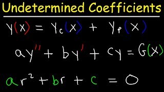
where a, b, c are constants and f(x) ≠ 0 is a known function (forcing function). The general solution of such an equation is:
y(x) = y_c(x) + y_p(x)
• y_c(x): Complementary function (solution of the homogeneous equation)
• y_p(x): Particular solution (also called particular integral)
The method of undetermined coefficients is a technique to find y_p(x), under certain conditions on f(x).
Detailed Explanation
The equation provided is a standard form of a second-order linear non-homogeneous differential equation. The function f(x) is what makes the equation non-homogeneous. When solving it, you'll calculate the complementary function from the associated homogeneous equation, which accounts for the natural properties of the system, and then find a particular solution that fits the specifics of the forcing function.
Examples & Analogies
Think of a bridge, where the stable structure represents the complementary function, while any additional movement caused by wind or traffic represents the particular integral. Together, they describe how the bridge behaves in a real-world scenario.
Conditions for Applying the Method
Chapter 3 of 4
🔒 Unlock Audio Chapter
Sign up and enroll to access the full audio experience
Chapter Content
This method works when the function f(x) is of the following types:
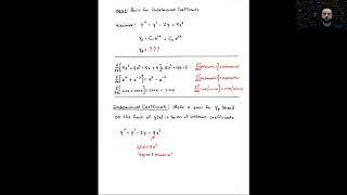
• Polynomial (e.g., f(x) = x² + 2x + 1)
• Exponential (e.g., f(x) = e^(kx))
• Sine or Cosine (e.g., f(x) = sin(ax), cos(bx))
• A product of the above (e.g., f(x) = xe^(kx), f(x) = x²sin(x))
It is not suitable for functions like ln(x), tan(x), or when f(x) is piecewise-defined or irregular.
Detailed Explanation
The method of undetermined coefficients is only applicable to specific types of functions. Understanding these types ensures that the method will produce valid solutions. If f(x) falls outside these types—like logarithmic functions or piecewise functionals—the method is inadequate, and alternative methods like Variation of Parameters should be used.
Examples & Analogies
Imagine trying to solve a puzzle where only specific pieces fit together. If you try to force a piece that doesn't belong, it won't fit. Similarly, for the method to work, we must ensure the pieces (functions) fit within the predefined categories.
Steps in the Method of Undetermined Coefficients
Chapter 4 of 4
🔒 Unlock Audio Chapter
Sign up and enroll to access the full audio experience
Chapter Content
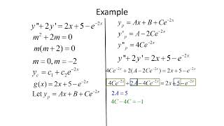
Step 1: Solve the Homogeneous Equation
ay′′ + by′ + cy = 0
Find the complementary function y_c by solving the auxiliary equation:
ar² + br + c = 0
The nature of roots (real and distinct, real and equal, or complex) determines the form of y_c.
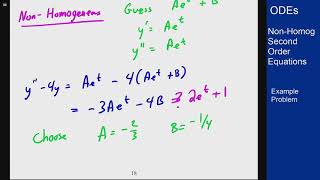
Step 2: Guess the Form of the Particular Integral y_p
Assume a trial solution for y based on the form of f(x), using undetermined coefficients.
Step 3: Modify Trial Solution if Needed
If any term in the trial solution already appears in y_c, multiply the entire trial solution by x (or x², if needed) to eliminate duplication. This adjustment is known as the "annihilator approach" or "repetition rule."
Step 4: Substitute and Determine Coefficients
Substitute the guessed y_p into the original non-homogeneous differential equation. Compare both sides and equate the coefficients of like terms to determine the unknown constants.
Step 5: Write the General Solution
y(x) = y_c(x) + y_p(x)
Detailed Explanation
This segment outlines the step-by-step process for using the method of undetermined coefficients:
1. Solve the homogeneous part to find the complementary function.
2. Make an educated guess for the particular integral.
3. Adjust your guess if it overlaps with the complementary function.
4. Substitute your guessed solution into the original equation and solve for any unknown coefficients.
5. Combine both components to write the general solution, which gives a comprehensive answer to the differential equation.
Examples & Analogies
Imagine a chef trying to create a new dish (the particular integral) while ensuring the dish complements the existing menu (the complementary function). The chef first makes a base dish, then tests new flavors, adjusts them if they clash with existing tastes (modifying the trial solution), and finally presents a refined dish to customers (writing the general solution).
Key Concepts
-
Linear Non-Homogeneous Differential Equation: The type of equations that involve a non-zero forcing term.
-
Complementary Function: The solution to the homogeneous part of the equation, essential for finding the general solution.
-
Particular Integral: Specific solution addressing the non-homogeneous components.
-
Undetermined Coefficients: A method of finding particular solutions by guessing based on the form of f(x).
Examples & Applications
Example of polynomial forcing function: y'' + y = x^2, leading to a particular solution of y_p = Ax^2 + Bx + C.
Example of an exponential forcing function: y'' - 3y' + 2y = e^x, with a particular integral involving a modification due to overlap.
Memory Aids
Interactive tools to help you remember key concepts
Rhymes
When you solve with coefficients undetermined, remember polynomial, exp, or sinusoidal - don’t feel burdened!
Stories
Imagine you're at a dance; the complementary function is dancing solo, while the particular integral must join in without stepping on toes – that's why we adjust!
Memory Tools
Remember the acronym 'STEP' for the method: Solve the homogeneous, Trial function guess, Eliminate duplication, and Substitute.
Acronyms
CUP - Complementary, Undetermined, Particular to remember the types of solutions.
Flash Cards
Glossary
- Linear NonHomogeneous Differential Equation
An equation involving derivatives of an unknown function and a known function that is not zero.
- Complementary Function
The solution to the corresponding homogeneous equation.
- Particular Integral
A specific solution to a non-homogeneous equation that fulfills the non-homogeneous part.
- Undetermined Coefficients
A method used for finding particular solutions based on the form of the non-homogeneous function.
- Auxiliary Equation
An algebraic equation obtained from the differential equation which is solved for its roots.
Reference links
Supplementary resources to enhance your learning experience.