
Steps in the Method of Undetermined Coefficients
Enroll to start learning
You’ve not yet enrolled in this course. Please enroll for free to listen to audio lessons, classroom podcasts and take practice test.
Interactive Audio Lesson
Listen to a student-teacher conversation explaining the topic in a relatable way.
Solving the Homogeneous Equation
🔒 Unlock Audio Lesson
Sign up and enroll to listen to this audio lesson

Let's start our discussion on the method of undetermined coefficients. The first step involves solving the homogeneous equation, which has the general form: ay'' + by' + cy = 0. Can anyone remind me what the corresponding auxiliary equation looks like?

Isn't it ar^2 + br + c = 0?
Excellent! That's correct, Student_1. The roots of this auxiliary equation will tell us about the complementary function, y_c. What are the types of roots we can have?

They can be real and distinct, real and equal, or complex!
Exactly! Remember, the nature of these roots will guide the form of y_c. A quick mnemonic to remember the types is: 'Real means distinct or equal, complex has a duo'—this highlights their characteristics. Now, who can give me an example of how we might solve this?

If the equation was y'' - 3y' + 2y = 0, we would find roots using the quadratic formula.
Right! And once we find those roots, we can express y_c appropriately. Great start; let’s move on.
Guessing the Form of the Particular Integral
🔒 Unlock Audio Lesson
Sign up and enroll to listen to this audio lesson

Now that we have our complementary function, let’s delve into step two, which is to guess the form of the particular integral, y_p. Based on the form of f(x), what trial solutions can we use?
If f(x) is a polynomial, we can try y_p = Ax^n + Bx^(n-1) + ... + C.
And for exponential functions like e^(kx), we simply use y_p = Ae^(kx).
Very good! For sine or cosine, we would use a combination of both: y_p = A cos(ax) + B sin(ax). These patterns are essential to remember! Now, why might we need to adjust our guess?
If any term in our guess matches the complementary function, we need to modify it to avoid repetition!
Precisely! This leads us to step three—let’s keep that in mind as we continue.
Substituting and Determining Coefficients
🔒 Unlock Audio Lesson
Sign up and enroll to listen to this audio lesson
In step four, we substitute our guessed y_p into the original differential equation. This process helps us find the unknown coefficients. Can someone explain how we might perform this substitution?
We differentiate y_p to find its derivatives, substitute these into the left-hand side, and then simplify!
Good! And what comes next after simplification?

We equate the coefficients of like terms from both sides to solve for our coefficients!
Exactly! Always remember to keep the equation balanced! To help remember, think of 'equating is relating!' Now let’s discuss how we finally write down the general solution.
Writing the General Solution
🔒 Unlock Audio Lesson
Sign up and enroll to listen to this audio lesson
Finally, in step five, how do we write the general solution after determining y_p?
We combine the complementary function y_c and the particular integral y_p together.
Correct! It's crucial to remember that the general solution is y(x) = y_c(x) + y_p(x). This simple formula can help in numerous applications. Does everyone see how these steps lead us through a complex process by breaking it down into manageable pieces?
Yes, and it’s really useful for practical problems in engineering!
Absolutely! In engineering, these solutions help predict behavior under various conditions. Recap everything we’ve learned today before moving to applications.
Introduction & Overview
Read summaries of the section's main ideas at different levels of detail.
Quick Overview
Standard
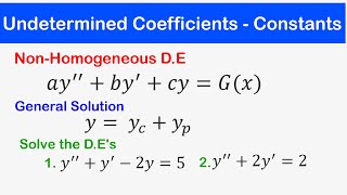
The section details five critical steps in applying the method of undetermined coefficients, including solving the homogeneous equation, guessing the form of the particular integral, modifying the trial solution if needed, determining coefficients by substitution, and forming the general solution. This methodology is crucial for civil engineers addressing real-world problems described by differential equations.
Detailed
In the method of undetermined coefficients, we tackle non-homogeneous linear differential equations with constant coefficients. The process begins with solving the complementary function from the associated homogeneous equation, followed by making an educated guess about the trial solution for the particular integral based on the known form of the non-homogeneous term. If the guessed function overlaps with the complementary function, we adjust it accordingly to ensure uniqueness. Subsequently, we substitute this trial solution into the original equation, equate coefficients to determine the unknown constants, and finally write down the complete general solution as the sum of the complementary function and particular integral. This method is especially beneficial in engineering applications where the functional forms of external forces are known and manageable.
Youtube Videos
![[Math][Differential Equations]-Method of Undetermined Coefficients-Concept and Beg Example Video](https://img.youtube.com/vi/HRS4Npq7uSA/mqdefault.jpg)


Audio Book
Dive deep into the subject with an immersive audiobook experience.
Step 1: Solve the Homogeneous Equation
Chapter 1 of 5
🔒 Unlock Audio Chapter
Sign up and enroll to access the full audio experience
Chapter Content
Solve the homogeneous equation: ay′′ + by′ + cy = 0. Find the complementary function y_c by solving the auxiliary equation: ar² + br + c = 0. The nature of roots (real and distinct, real and equal, or complex) determines the form of y_c.
Detailed Explanation
In this first step, we begin by solving the associated homogeneous equation, which is an equation without the non-homogeneous term. The goal is to find the complementary function, y_c. To do this, we write down the auxiliary equation (which is derived from the homogeneous equation) and solve for the roots. These roots can either be real and different, real and the same, or complex. Each type of root gives a different form for y_c. If the roots are real and distinct, for example, the complementary function takes the form of a linear combination of exponentials. If the roots are complex, it will include sine and cosine functions.
Examples & Analogies
You can think of finding the complementary function as discovering the basic modes of vibration of a musical instrument. Different instruments produce different tones based on their construct (analogous to the nature of the roots) — for instance, a guitar and a violin can both vibrate but produce distinct sounds based on their design.
Step 2: Guess the Form of the Particular Integral y_p
Chapter 2 of 5
🔒 Unlock Audio Chapter
Sign up and enroll to access the full audio experience
Chapter Content
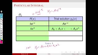
Assume a trial solution for y_p based on the form of f(x), using undetermined coefficients. The forms of trial solutions are:
- P(x) (polynomial of degree n) => y_p = Ax^n + Bx^{n-1} + ... + C
- e^(kx) => y_p = Ae^(kx)
- sin(ax), cos(ax) => y_p = Acos(ax) + Bsin(ax)
- x^m e^(kx) => y_p = (Ax^m + ... + C)e^(kx)
- e^(kx)sin(ax), e^(kx)cos(ax) => y_p = e^(kx)(Acos(ax) + Bsin(ax)).
Detailed Explanation
In this step, we propose a form for the particular integral solution, y_p, based on the type of the forcing function f(x). We create a trial function that mimics the same structure as f(x). For example, if f(x) is a polynomial of degree n, our trial solution will be a polynomial of the same degree with undetermined coefficients (A, B, C, etc.). This trial function will allow us to approximate the response of the system to the external forces represented by f(x). The trial form changes based on whether f(x) is polynomial, exponential, or sinusoidal.
Examples & Analogies
Imagine you're trying to predict the future sales of a product based on past performance. If sales data shows a quadratic trend, you'd build a model (a polynomial form) that fits that trend to forecast future sales. In this method, we craft our 'guess' in a similar way, based on the visible trend indicated by f(x).
Step 3: Modify Trial Solution if Needed
Chapter 3 of 5
🔒 Unlock Audio Chapter
Sign up and enroll to access the full audio experience
Chapter Content
If any term in the trial solution already appears in y_c, multiply the entire trial solution by x (or x², if needed) to eliminate duplication. This adjustment is known as the 'annihilator approach' or 'repetition rule.'
Detailed Explanation
In this step, we need to ensure that our trial solution for y_p does not overlap with the complementary function y_c. If it does, we modify the trial solution by multiplying it by the smallest power of x necessary to eliminate that overlap. This technique is referred to as the 'annihilator approach,' and it helps ensure that the different parts of our solution are linearly independent. This adjustment is critical because if we did not make this change, we would not properly account for the effects of the non-homogeneous part on the system.
Examples & Analogies
Think of stacking books on a shelf. If one book is too similar in size to another already on the shelf, it wouldn't fit well without creating clutter. So you might stack it on top of the other, using a box underneath to create space. In the context of the trial solution, we create space by multiplying our guessed function to avoid 'clutter' or duplicates with y_c.
Step 4: Substitute and Determine Coefficients
Chapter 4 of 5
🔒 Unlock Audio Chapter
Sign up and enroll to access the full audio experience
Chapter Content
Substitute the guessed y_p into the original non-homogeneous differential equation. Compare both sides and equate the coefficients of like terms to determine the unknown constants.
Detailed Explanation
During this crucial step, we substitute our modified trial solution y_p back into the original non-homogeneous differential equation. Once substituted, we compare the left-hand side and the right-hand side of the equation. By aligning like terms, we can solve for the unknown coefficients (such as A, B, C) in our trial solution. This process of equating coefficients helps establish the exact influence of the non-homogeneous term on the solution.
Examples & Analogies
Consider a recipe where you need to mix ingredients to achieve the right taste. After guessing the ratio of sugar to flour, you taste the mixture (substitution). If it's too sweet, you adjust the sugar content until it matches your ideal flavor (comparing and adjusting coefficients). In mathematics, this adjustment helps us refine our guess to fit the equation perfectly.
Step 5: Write the General Solution
Chapter 5 of 5
🔒 Unlock Audio Chapter
Sign up and enroll to access the full audio experience
Chapter Content
Finally, the general solution is obtained by combining the complementary function and the particular solution: y(x) = y_c(x) + y_p(x).
Detailed Explanation
In the final step, we combine the solutions found in the previous steps. The general solution to the non-homogeneous differential equation is created by adding the complementary function y_c (found from the homogeneous part) to the particular solution y_p (derived through our guesses). This gives us a complete solution that incorporates both the natural behavior of the system and the effect of the external forces.
Examples & Analogies
This step is like putting together a complete puzzle after finding individual pieces. Each piece represents a different aspect: the complementary function captures the inherent characteristics of the system, while the particular solution shows how it reacts to external influences. Together, they create the full picture of the situation you are analyzing.
Key Concepts
-
Complementary Function: The solution to the homogeneous differential equation that helps form the general solution.
-
Particular Integral: The specific solution that addresses the non-homogeneous part of the equation, often requiring guessing and substitution.
-
Trial Solution: The predicted form of the particular integral based on known function types.
Examples & Applications
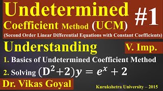
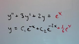
Example 1: For the equation y'' - 3y' + 2y = e^x, the corresponding auxiliary equation is r^2 - 3r + 2 = 0, leading to roots 1 and 2.
Example 2: In y'' + y = x^2, the particular integral is guessed as y_p = Ax^2 + Bx + C.
Memory Aids
Interactive tools to help you remember key concepts
Rhymes
Solve the homogenous to find the base, guess the particular to give it pace, modify if they share a face!
Stories
Imagine a chef creating a special dish. He first prepares a classic base (the complementary function) but must guess the right secret ingredient (the particular integral). If someone accidentally puts in the same spice as the base, the chef must find a new way to add flavor!
Memory Tools
Solve, Guess, Modify, Substitute, Generalize (SGMSG).
Acronyms
C-P-TS (Complementary Function, Particular Integral, Trial Solution) to remember the order of solutions.
Flash Cards
Glossary
- Homogeneous Equation
A differential equation where the non-homogeneous term is zero.
- Complementary Function (y_c)
The solution to the homogeneous equation.
- Particular Integral (y_p)
The specific solution to the non-homogeneous part of the equation.
- Auxiliary Equation
The polynomial equation obtained by substituting y and its derivatives into the homogeneous equation.
- Trial Solution
An assumed form of the particular integral based on the non-homogeneous term.
Reference links
Supplementary resources to enhance your learning experience.