
Step 2: Guess the Form of the Particular Integral
Enroll to start learning
You’ve not yet enrolled in this course. Please enroll for free to listen to audio lessons, classroom podcasts and take practice test.
Interactive Audio Lesson
Listen to a student-teacher conversation explaining the topic in a relatable way.
Introduction to Particular Integral
🔒 Unlock Audio Lesson
Sign up and enroll to listen to this audio lesson

Today, we will explore how to guess the form of the particular integral, or y_p, in our differential equations. This step is crucial because the form we choose depends largely on the non-homogeneous term, f(x).

What do you mean by non-homogeneous term?
Great question! The non-homogeneous term is the part of the equation that forces it away from being homogeneous—essentially it’s what you’re adding to the equation, like forces in structural engineering.

So, f(x) can be different types of functions, right?
Exactly! It can be a polynomial, exponential, or even sine and cosine functions. We define the type in our guess for y_p.

How do we know what form to pick?
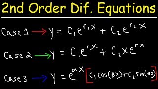
We follow a specific set of trial solutions based on the type of f(x). For example, if f(x) is a polynomial of degree n, we'll guess y_p to be of the form Ax^n + Bx^{n-1} + ... + C.

What happens if it overlaps with the complementary function?
Excellent! In such cases, we need to modify our trial solution by multiplying it by x or x² to remove the duplication.
Today we solidified how crucial the guess for y_p is when dealing with different forms of f(x).
Determining the Trial Solution
🔒 Unlock Audio Lesson
Sign up and enroll to listen to this audio lesson

Now, let's break down the specific cases for trial solutions. If f(x) is an exponential function like e^(kx), how would we guess y_p?
Wouldn’t it be Ae^(kx)?
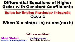
Correct! And what about sine or cosine functions?
That would be A*cos(ax) + B*sin(ax).
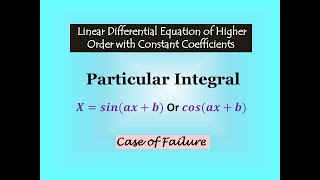
Wait, isn’t there a chance of overlap with the complementary function here as well?
Absolutely! If either function overlaps with y_c, then we would need to adjust again by multiplying by x or higher powers of x.
What about products like x*e^(kx)?
For that, we generally guess y_p = (Ax^m + ... + C)e^(kx), with m indicating the degree of the polynomial part.
Today, we practiced identifying different trial solution forms for various types of functions, reinforcing our understanding of this crucial method in solving for y_p.
Adjusting for Repetition
🔒 Unlock Audio Lesson
Sign up and enroll to listen to this audio lesson
Next, let's talk about the modification step for our trial solution when there’s a duplication with y_c. How do we deal with that?
We would multiply the entire trial solution by x or x²?
Exactly! This is known as the 'annihilator approach'. It allows us to ensure our particular integral is independent of the complementary function.
So, if y_c included e^(2x), we couldn’t guess Ae^(2x)?
Right! In that case, we would use Ax*e^(2x) instead. Can anyone give me another case? Like if we have duplicated terms in y_c?
If e^(2x) appears more than once, we would try Ax²*e^(2x).
Perfect! Understanding this adjustment is critical for ensuring our guessed solutions work in the context of the differential equation.
Today we reinforced how to handle duplications effectively and how this can lead to the successful determination of our particular integral.
Introduction & Overview
Read summaries of the section's main ideas at different levels of detail.
Quick Overview
Standard
It covers the steps required to determine the trial solution for the particular integral based on the type of the non-homogeneous term, including special considerations for duplication with the complementary function, thus guiding the method of solution.
Detailed
In this crucial step of the undetermined coefficients method, we focus on guessing the form of the particular integral (denoted as y_p). The structure of y_p depends on the nature of the non-homogeneous term, f(x), subjected to certain predefined cases, such as polynomials, exponentials, sines, and cosines. This method is particularly helpful in civil engineering applications, where functions follow specific typical behaviors. Further, if components of y_p overlap with the complementary function (y_c), adjustments are necessary to account for this repetition, ensuring that we have a valid form for y_p. This section is essential in bridging the theoretical framework with practical applications in engineering challenges, thereby facilitating the solution of complex differential equations.
Youtube Videos


Key Concepts
-
Particular Integral: The specific solution derived in the undetermined coefficients method based on the forcing function.
-
Guessing the Form: The initial assumption of y_p is critical and depends on f(x).
-
Duplication Handling: Special adjustments are necessary when y_p overlaps with the complementary function.
Examples & Applications
If f(x) = x^2, the trial solution would be y_p = Ax^2 + Bx + C.
If f(x) = e^(2x), then y_p = Ae^(2x), adjusting if e^(2x) appears in y_c.
Memory Aids
Interactive tools to help you remember key concepts
Rhymes
For the integral you must guess, ensure you choose the right mess; polynomials, sine, and more, adjust with x if you want to score!
Stories
Imagine you're a detective guessing the right trail (y_p) from several clues (f(x)); if two clues match, you adjust your path (multiply by x) to find the right answer!
Memory Tools
G for Guess, A for Adjust — remember 'GA' for the steps needed in y_p.
Acronyms
T.S. (Trial Solution)
for Type
for Solve. Just remember the TS for types of functions to guess correctly.
Flash Cards
Glossary
- Particular Integral
A specific solution to a non-homogeneous differential equation that satisfies the equation for a particular forcing function.
- Complementary Function
The general solution to the associated homogeneous equation derived from the differential equation.
- NonHomogeneous Term
The part of the differential equation that does not include the dependent variable or its derivatives.
- Trial Solution
An assumed form of the particular integral that will be modified and adjusted based on the properties of the function f(x).
- Duplcication
Occurrence where terms in the trial solution overlap with components in the complementary function.
Reference links
Supplementary resources to enhance your learning experience.