
Comparison of Methods
Enroll to start learning
You’ve not yet enrolled in this course. Please enroll for free to listen to audio lessons, classroom podcasts and take practice test.
Interactive Audio Lesson
Listen to a student-teacher conversation explaining the topic in a relatable way.
Overview of Numerical Methods
🔒 Unlock Audio Lesson
Sign up and enroll to listen to this audio lesson

Today, we're going to compare different numerical methods. Can anyone first name a few numerical techniques we've learned?

We learned about finite difference methods and Newton-Cotes formulas!
Excellent! How about we start with finite difference methods? These are commonly used for approximating derivatives. Can someone explain how these work?

They use discrete points to estimate derivatives, right?
That's correct! We have different types: forward, backward, and central differences. Remember the acronym 'FBC' for this! Now, what do you think are the pros and cons of finite differences?

It's easy to implement but less accurate if the step size is large.
Spot on! Let's summarize: Finite differences are simple to implement and work well with smaller step sizes.
Newton-Cotes Formulas
🔒 Unlock Audio Lesson
Sign up and enroll to listen to this audio lesson

Next, let’s discuss Newton-Cotes formulas. Can anyone tell me what they are used for?
They approximate integrals using polynomials!
Exactly! The trapezoidal rule is the first-order method. Who can describe how it works?
It connects points with straight lines to estimate the area.
Well said! Remember, its error decreases as O(h²). What about Simpson's rule?

It uses quadratic polynomials and has faster convergence, O(h⁴).
Excellent observation! So, remember: Simpson’s rule requires an even number of intervals and is more accurate than the trapezoidal rule.
Gaussian Quadrature
🔒 Unlock Audio Lesson
Sign up and enroll to listen to this audio lesson
Finally, let's discuss Gaussian quadrature. Who can define it for us?
It’s a method that uses optimized points to approximate integrals more accurately.
Correct! And why do we prefer Gaussian quadrature over Newton-Cotes formulas?
Because it can achieve higher accuracy with fewer points!
Right again! It’s especially effective for smooth functions. Don’t forget that it can be computationally expensive!
So, is it usually better than Newton-Cotes then?
Not always, but for functions where we expect smooth behavior, Gaussian quadrature has significant advantages!
Comparative Summary
🔒 Unlock Audio Lesson
Sign up and enroll to listen to this audio lesson
Let's compare what we've discussed. Could someone summarize the convergence and complexity for finite difference methods?
They converge linearly and are low in computational complexity!
Great! Moving on to Newton-Cotes. Who can tell me about its error rates?
Trapezoidal has O(h²) and Simpson's has O(h⁴)!
Exactly! And for Gaussian quadrature?
It’s high accuracy with exponential convergence but more complex.
Excellent summary! Always remember to choose based on your required accuracy and computational resources.
Introduction & Overview
Read summaries of the section's main ideas at different levels of detail.
Quick Overview
Standard
In this section, we analyze the different numerical methods for differentiation and integration. We compare finite difference methods, Newton-Cotes formulas, and Gaussian quadrature based on their convergence rates, computational complexity, advantages, and disadvantages, providing a clear overview of which method may be suitable for specific scenarios.
Detailed
Detailed Summary
In this section, we systematically compare various numerical methods used for differentiation and integration, namely finite difference methods, Newton-Cotes formulas, and Gaussian quadrature. The comparison focuses on several criteria:
- Convergence Rate: This indicates how quickly a method approaches the exact solution as the number of data points increases or as the step size decreases.
- Finite Difference Methods converge linearly.
- Newton-Cotes formulas exhibit quadratic (trapezoidal rule) or quartic (Simpson's rule) convergence.
- Gaussian Quadrature achieves exponential convergence.
- Computational Complexity: This involves the number of function evaluations needed (or computational effort) to apply the method effectively.
- Finite Difference Methods and Newton-Cotes only require one point (or segment).
- Gaussian Quadrature often requires two or more points.
- Pros and Cons:
- Finite Difference Methods: Simple to implement but accuracy depends on the step size chosen.
- Trapezoidal Rule: Easy to use, but convergence is slower compared to Simpson’s rule.
- Simpson's Rule: Offers faster convergence with a requirement for an even number of intervals.
- Gaussian Quadrature: Highly accurate and efficient for smooth functions, but more computationally complex.
The careful selection among these methods is crucial depending on the problem requirements, desired accuracy, and available computational resources.
Youtube Videos

Audio Book
Dive deep into the subject with an immersive audiobook experience.
Overview of Comparison
Chapter 1 of 5
🔒 Unlock Audio Chapter
Sign up and enroll to access the full audio experience
Chapter Content
Method | Convergence Rate | Number of Points | Computational Complexity | Pros | Cons
Detailed Explanation
This chunk introduces the format in which various numerical methods will be evaluated. It specifies five key dimensions for comparison, including convergence rate, number of points required for computations, computational complexity, and the advantages ('Pros') and disadvantages ('Cons'). Understanding this table will help students grasp how different methods stack up against one another and under what criteria.
Examples & Analogies
Think of comparing different types of vehicles. The table is like a comparison chart that lists various vehicles' speed (convergence rate), how many passengers they can seat (number of points), how much fuel they consume (computational complexity), the comfort they provide (pros), and their drawbacks (cons).
Finite Difference Method
Chapter 2 of 5
🔒 Unlock Audio Chapter
Sign up and enroll to access the full audio experience
Chapter Content
| Finite Difference | Linear | 1 (for each derivative) | Low | Simple, easy to implement | Accuracy depends on step size |
Detailed Explanation
The finite difference method approximates derivatives using simple calculations based on the function values at specific points. It's linear in convergence, meaning that the error decreases in a straightforward manner as the step size decreases. This method only requires one function evaluation per derivative calculated and is relatively easy to apply. However, the accuracy can vary depending on the chosen step size, requiring careful selection.
Examples & Analogies
Imagine trying to find the slope of a hill by taking quick measurements at various points. If you only take a few measurements (step size) far apart, your estimate may be off. But if you gather many measurements close together, you’ll get a much better idea of the hill’s slope. The finite difference method is similar; gathering 'more data' (smaller step size) leads to improved accuracy.
Trapezoidal Rule
Chapter 3 of 5
🔒 Unlock Audio Chapter
Sign up and enroll to access the full audio experience
Chapter Content
| Trapezoidal Rule | O(h^2) | 1 (for each segment) | Low | Easy to implement | Slow convergence |
Detailed Explanation
The trapezoidal rule is a numerical integration technique that approximates the area under a curve by dividing it into segments and forming trapezoids. The convergence rate is proportional to O(h²), indicating that the error decreases quadratically as the step size shrinks. While it's straightforward to implement and requires one function evaluation per segment, its convergence can be slower compared to other methods.
Examples & Analogies
Think about trying to calculate the area of a park by dividing it into small trapezoidal sections instead of squares. Using trapezoids might yield a close estimate of the park's area, but if the sections are too far apart, the estimate becomes less accurate. The trapezoidal rule works similarly and needs careful segmentation to improve accuracy.
Simpson's Rule
Chapter 4 of 5
🔒 Unlock Audio Chapter
Sign up and enroll to access the full audio experience
Chapter Content
| Simpson’s Rule | O(h^4) | 1 (for each segment) | Low to moderate | Faster than trapezoidal | Requires an even number of intervals |
Detailed Explanation
Simpson's rule improves over the trapezoidal rule by using quadratic polynomials to approximate the area under a curve. Its error rate is considerably better at O(h^4), meaning it requires fewer segments or points for the same accuracy level. However, it does necessitate that the number of intervals be even, which can be a limitation in practical situations.
Examples & Analogies
If calculating the area of a curvy garden using different shapes, using straight lines gives a basic estimate, but using curves (like parabolas) will yield a more accurate area measurement. Simpson's rule uses these smooth curves for better results but requires an equal number of 'sections' to fit properly.
Gaussian Quadrature
Chapter 5 of 5
🔒 Unlock Audio Chapter
Sign up and enroll to access the full audio experience
Chapter Content
| Gaussian Quadrature | Exponential | 2 or more | High | Very accurate | Computationally expensive |
Detailed Explanation
Gaussian Quadrature is a sophisticated method for numerical integration that achieves high accuracy by evaluating the function at strategically chosen points. Unlike previous methods, which rely on evenly spaced points, Gaussian quadrature uses a weighted sum of function values at optimal locations. It's highly accurate but typically requires more computational resources due to the complexity of the calculations.
Examples & Analogies
Think of a precision machine trying to perfectly cut a shape. While simple machines might use basic tools at regular intervals, the precision machine applies advanced techniques to target areas where cuts will matter most, leading to superior results. Gaussian Quadrature similarly prioritizes specific points to ensure maximum accuracy, albeit at the cost of requiring more advanced calculations.
Key Concepts
-
Finite Difference Methods: Used to approximate derivatives using discrete points.
-
Newton-Cotes Formulas: A family of polynomials for estimating integrals based on interpolation.
-
Gaussian Quadrature: A method for integrating functions with high accuracy using optimal points.
Examples & Applications
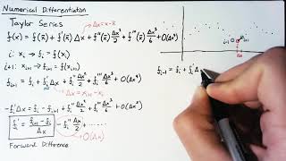
An example of the finite difference method would be using the forward difference formula to estimate the derivative of f(x) at x = a by using values at a and a+h.
Using Simpson's rule, one could approximate the integral of f(x) from a to b by applying the formula that incorporates both odd and even indexed function values.
Memory Aids
Interactive tools to help you remember key concepts
Rhymes
If you want to derive, finite differences will thrive; they take steps to ensure you stay alive!
Stories
Imagine you are a sculptor shaping a curve. With finite differences, each point you chisel must lead to the next, showing the shape's true line.
Memory Tools
For Newton-Cotes: T for Trapezoidal, S for Simpson's, H for Higher-order. Remember TSH to address how we fit curves!
Acronyms
FNG
Finite difference is Simple
Newton-Cotes is Polishing
Gaussian is Golden. FNG for methods hierarchy!
Flash Cards
Glossary
- Finite Difference Methods
Numerical methods for approximating derivatives using discrete data points.
- NewtonCotes Formulas
A family of methods for numerical integration based on interpolating polynomials.
- Gaussian Quadrature
A numerical integration method that uses optimized nodes for more accurate approximations.
- Convergence Rate
The speed at which a numerical method approaches the exact solution as the number of points increases.
- Computational Complexity
The amount of computational resources (e.g., function evaluations) required to implement a method.
Reference links
Supplementary resources to enhance your learning experience.