
Numerical Differentiation and Integration
Enroll to start learning
You’ve not yet enrolled in this course. Please enroll for free to listen to audio lessons, classroom podcasts and take practice test.
Interactive Audio Lesson
Listen to a student-teacher conversation explaining the topic in a relatable way.
Introduction to Numerical Differentiation
🔒 Unlock Audio Lesson
Sign up and enroll to listen to this audio lesson

Today, we're diving into numerical differentiation! Can anyone tell me what differentiation means?

Isn't differentiation how we find the slope of a function?
Exactly! But sometimes we can't find the derivative analytically. That's where numerical methods come in. Can anyone think of a situation where we might need this?

If we have experimental data, we might not have a function to differentiate.
Good point! So we use methods like finite difference for approximating the derivative. Remember the acronym FBC: Forward, Backward, and Central differences?

Right! Forward uses the next point, backward uses the previous one, and central uses both.
Great! To recap, numerical differentiation helps us find slopes when we can't rely on an explicit function. Let’s move on to how we calculate these differences.
Finite Difference Methods
🔒 Unlock Audio Lesson
Sign up and enroll to listen to this audio lesson

Let’s delve deeper into finite difference methods. Who can explain the forward difference method?

It approximates the derivative using the current point and the next point, right?
Correct! The formula is `f'(x) ≈ (f(x+h) - f(x))/h`. What are some pros and cons of this method?
It's easy to implement but could be less accurate if h is too large!
Well stated! Now, let's discuss the central difference. Why might it be more advantageous?
Because it uses points on both sides, making it more accurate!
Exactly! Remember, its error decreases quadratically. Always choose the method based on your data!
Numerical Integration Basics
🔒 Unlock Audio Lesson
Sign up and enroll to listen to this audio lesson
Now, let's shift to numerical integration. Who can define it for us?
It's used to calculate the area under a curve when we can't integrate analytically!
That's right! A common method is the Trapezoidal Rule. Can someone explain how it works?
It connects the points with straight lines to estimate the area!
Perfect! And how would we express the error in this rule?
The error is proportional to O(h²)!
Very good! Now let's discuss Simpson's Rule. What’s the key difference?
It uses parabolas to fit the data instead of straight lines!
Exactly! And it has an error of O(h⁴). This makes it important for smoother functions.
Gaussian Quadrature
🔒 Unlock Audio Lesson
Sign up and enroll to listen to this audio lesson
Let's introduce Gaussian Quadrature. Anyone familiar with this method?
Isn’t it known for using specific nodes for better accuracy?
Indeed! It uses weighted sums at strategically chosen points. Why do you think this is beneficial?
It can achieve high accuracy with fewer points compared to other methods!
Absolutely! And remember the example we discussed with the function e^(-x²)?
Yes! Using 2-point Gaussian quadrature was more accurate than other methods!
Excellent! This juxtaposition emphasizes how method selection impacts results.
I see how critical it is to choose the right method now!
Comparative Overview of Methods
🔒 Unlock Audio Lesson
Sign up and enroll to listen to this audio lesson
Finally, let’s do a quick comparison of all methods discussed. What are the key takeaways?
Finite differences are straightforward but can have cumulative error.
Correct! And Newton-Cotes has an order-based error while Gaussian Quadrature is more efficient.
So the choice of method relies on the required accuracy and data characteristics?
Exactly! Always consider your specific application and available computational resources.
This was very insightful! Thank you for explaining the relations between all methods.
You're welcome! Remember, understanding these methods enhances your problem-solving skills in real-world scenarios.
Introduction & Overview
Read summaries of the section's main ideas at different levels of detail.
Quick Overview
Standard
Numerical differentiation and integration are crucial for approximating derivatives and integrals of functions when analytical solutions are impractical. The section covers various methods such as finite difference methods, Newton-Cotes formulas, and Gaussian quadrature, highlighting their applications and accuracies.
Detailed
Detailed Summary of Numerical Differentiation and Integration
Numerical differentiation and integration are techniques utilized to estimate derivatives and integrals of functions that cannot be easily solved analytically. These methods are particularly useful in fields like engineering, physics, and economics, where real-world data may not be represented in closed-form.
Numerical Differentiation
Numerical differentiation approximates the derivative of a function using discrete data points. The most common approach is the finite difference method, which involves:
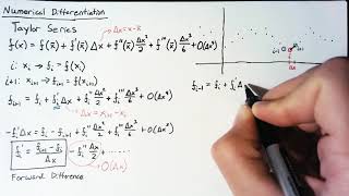
- Forward Difference: Uses the function value at a point and a small step forward to approximate the derivative. Formula: f'(x) ≈ (f(x+h) - f(x))/h.
- Backward Difference: Uses a small step backward. Formula: f'(x) ≈ (f(x) - f(x-h))/h.
- Central Difference: Utilizes both forward and backward points for a more accurate estimate. Formula: f'(x) ≈ (f(x+h) - f(x-h))/(2h).
The accuracy of these methods varies, where the forward and backward differences yield linear error O(h), and the central difference has a quadratic error O(h²).
Numerical Integration
This involves approximating an integral using numerical methods, especially when analytical solutions are unavailable.
- Newton-Cotes Formulas: Include methods such as the Trapezoidal Rule and Simpson's Rule.
- Trapezoidal Rule: Approximates the integral using straight lines between points. Its error is O(h²).
- Simpson’s Rule: Utilizes quadratic polynomials for a more precise approximation, reducing the error to O(h⁴).
Gaussian Quadrature
This method aims for higher accuracy by strategically choosing points (nodes) for evaluation, leading to effective integral approximations with weighted sums of function values.
- Example: Integrating the function f over an interval using Gaussian quadrature often results in superior accuracy compared to Newton-Cotes methods.
Choosing the appropriate numerical method depends on the specific problem, desired accuracy, and available computational resources.
Youtube Videos

Audio Book
Dive deep into the subject with an immersive audiobook experience.
Introduction to Numerical Methods
Chapter 1 of 13
🔒 Unlock Audio Chapter
Sign up and enroll to access the full audio experience
Chapter Content
Numerical differentiation and integration are fundamental techniques used in computational mathematics to approximate the derivative or integral of a function when an analytical solution is difficult or impossible to obtain. These techniques are used extensively in engineering, physics, economics, and many other fields, especially for solving real-world problems that involve data points or functions that are not easily expressed in closed-form. This chapter explores the main numerical techniques used for differentiation and integration, including finite difference methods, Newton-Cotes formulas, and Gaussian quadrature.
Detailed Explanation
Numerical differentiation and integration are key processes used when functions are complex and cannot be easily solved with traditional analytical methods. These techniques help in approximating the derivative (how a function changes) or the integral (the area under a curve) using numerical data instead of exact equations. This is particularly helpful in various fields like engineering and physics where we often have experimental data points that do not follow a simple mathematical formula. The chapter outlines different methods such as finite differences for derivatives and Newton-Cotes for integration.
Examples & Analogies
Think about a weather app that predicts temperatures. The app collects data points (like temperatures recorded each hour) to estimate the temperature at any given time (differentiation) or to calculate the total temperature change over a day (integration). Without numerical techniques, it’s challenging to get accurate predictions from discrete data.
Numerical Differentiation
Chapter 2 of 13
🔒 Unlock Audio Chapter
Sign up and enroll to access the full audio experience
Chapter Content
Numerical differentiation refers to the process of approximating the derivative of a function based on discrete data points. Since derivatives are defined as the limit of a difference quotient, numerical differentiation involves approximating this quotient with values of the function at a discrete set of points.
Detailed Explanation
Numerical differentiation deals with estimating how fast a function is changing at a certain point based on known data. Instead of looking for an exact formula, we take points around the value of interest and calculate the change between them. This gives us a practical way to find derivatives without needing the exact equation of the function.
Examples & Analogies
Imagine you are monitoring the speed of a car. If you record its position every second, you can figure out how fast it's going by calculating the difference in position between two consecutive seconds. This difference quotient is what numerical differentiation does with functions.
Finite Difference Methods
Chapter 3 of 13
🔒 Unlock Audio Chapter
Sign up and enroll to access the full audio experience
Chapter Content
Finite difference methods are the most commonly used approach for approximating derivatives in numerical methods. These methods estimate the derivative by using function values at discrete points and are categorized based on the number of points used for the approximation. 1. Forward Difference: Approximates the derivative using the function value at a point and a small step forward.
f′(x)≈f(x+h)−f(x)h
- Pros: Simple and easy to implement.
- Cons: Less accurate; errors can accumulate if h is too large. 2. Backward Difference: Uses the function value at the point and a small step backward.
f′(x)≈f(x)−f(x−h)h
- Pros: Works well for data that is given in reverse order.
- Cons: Less accurate than central differences. 3. Central Difference: Uses function values at both a small step forward and backward to compute a more accurate approximation of the derivative.
f′(x)≈f(x+h)−f(x−h)2h
- Pros: More accurate than forward and backward differences for the same step size.
- Cons: Requires data points on both sides of the point of interest.
Detailed Explanation
Finite difference methods are techniques for estimating derivatives using values from a function evaluated at specific points. There are three main approaches: Forward Difference uses the point of interest and a point ahead, Backward Difference uses the point of interest and a point behind, while Central Difference averages points from both sides. Each method has its strengths and weaknesses concerning ease of use and accuracy, with Central Difference generally offering better precision.
Examples & Analogies
Think of a doctor monitoring heart rates. If the doctor checks the pulse every few seconds, they can estimate how quickly the heart rate changes depending on the rhythm of the heart. Similarly, using data from several points around the desired time, we can estimate the rate of change of a function.
Error in Finite Difference Methods
Chapter 4 of 13
🔒 Unlock Audio Chapter
Sign up and enroll to access the full audio experience
Chapter Content
The error in finite difference methods depends on the step size h and the method used: ● Forward/Backward Difference: The error is O(h), meaning the error decreases linearly as h decreases. ● Central Difference: The error is O(h²), which means it decreases quadratically with decreasing h.
Detailed Explanation
The accuracy of the finite difference methods is influenced by the size of the step (h) used in calculations. In Forward and Backward Differencing, as the step size decreases, the error reduces at a linear rate. In contrast, Central Differencing achieves a better error reduction rate since its error term decreases quadratically, meaning it becomes significantly more accurate as you refine your step size.
Examples & Analogies
Consider a painter working with a canvas. If they use a large brush (large h), the details can be missed (high error). If they switch to a smaller brush (small h), they capture more details. Central difference is like using a fine brush, capturing even finer details in the artwork.
Numerical Integration
Chapter 5 of 13
🔒 Unlock Audio Chapter
Sign up and enroll to access the full audio experience
Chapter Content
Numerical integration refers to the process of approximating the integral of a function when an exact analytical solution is difficult or unavailable. Numerical methods are used to estimate the area under a curve based on discrete data points.
Detailed Explanation
Numerical integration is crucial when the exact area under a curve is hard to find analytically. It estimates the total area using numerical data points instead of trying to find the area using a formula. This is particularly useful in applications where the underlying function is known only at specific intervals.
Examples & Analogies
Imagine trying to measure the water that flows into a pool using a series of small buckets. Even if you can't get a perfect count of the total water volume, by summing the water in each bucket (data points), you can get a good estimate of the total water volume (integral).
Newton-Cotes Formulas
Chapter 6 of 13
🔒 Unlock Audio Chapter
Sign up and enroll to access the full audio experience
Chapter Content
The Newton-Cotes formulas are a family of methods for numerical integration based on interpolating the integrand using polynomials. These methods approximate the integral by fitting a polynomial to the data and integrating that polynomial. 1. Trapezoidal Rule (First-Order Newton-Cotes Formula): The trapezoidal rule approximates the integral by using a straight line (linear interpolation) between adjacent points. 2. I=∫abf(x) dx≈h2[f(x0)+2∑i=1n−1f(xi)+f(xn)] I = ∫ab f(x) dx ≈ h/2 [f(x₀) + 2∑(f(xᵢ)) + f(xₙ)] - Pros: Simple and efficient for smooth functions. - Cons: Error decreases linearly with the number of points. 3. Simpson's Rule (Second-Order Newton-Cotes Formula): Simpson’s rule approximates the integral using quadratic polynomials to fit the data. 4. I=∫abf(x) dx≈h3[f(x0)+4∑i oddf(xi)+2∑i evenf(xi)+f(xn)] I = ∫ab f(x) dx ≈ h/3 [f(x₀) + 4∑(f(xᵢ odd)) + 2∑(f(xᵢ even)) + f(xₙ)] - Pros: More accurate than the trapezoidal rule for the same number of points. The error decreases as O(h⁴). - Cons: Requires an even number of intervals and works best for smooth functions.
Detailed Explanation
Newton-Cotes formulas consist of polynomial fitting to estimate the integral of functions through numerical methods. The Trapezoidal Rule uses straight lines to estimate the area under curves, while Simpson's Rule employs parabolas, providing greater accuracy. Each method relies on how many points you include, and while they are simple to use, their accuracy also depends on the chosen step size.
Examples & Analogies
Think of a farmer estimating the area of irregular crops by stretching a sheet of flexible plastic over the crops. If the plastic is flat (Trapezoidal Rule), it may not fit perfectly, but if you mold it to fit better (Simpson's Rule), you get a more accurate area estimate.
Error in Newton-Cotes Formulas
Chapter 7 of 13
🔒 Unlock Audio Chapter
Sign up and enroll to access the full audio experience
Chapter Content
The error in the trapezoidal rule is proportional to O(h²). The error in Simpson’s rule is proportional to O(h⁴), making it more accurate for the same number of intervals. Both methods improve accuracy as the step size h is reduced, though higher-order formulas increase the computational cost.
Detailed Explanation
Both the Trapezoidal and Simpson's methods will yield errors that decrease as the step size (h) is reduced. However, the decrease rate differs significantly: Simpson’s Rule enjoys a faster accuracy improvement at O(h⁴), while Trapezoidal only improves at O(h²). This means that while both methods become more precise with a smaller h, Simpson's method is more fundamentally accurate for integrals.
Examples & Analogies
Returning to the farmer, if he measures smaller portions of his crops (smaller h), he's bound to get a better estimate of his total area. If he uses a sophisticated measuring method instead of a basic one, he might get an even better estimate in less time.
Gaussian Quadrature
Chapter 8 of 13
🔒 Unlock Audio Chapter
Sign up and enroll to access the full audio experience
Chapter Content
Gaussian quadrature is a more accurate method for numerical integration that aims to maximize the number of points used in the integral while minimizing the associated error. Unlike Newton-Cotes formulas, Gaussian quadrature uses non-uniformly spaced points that are chosen to optimize the approximation of the integral.
Detailed Explanation
Gaussian quadrature enhances the method of numerical integration by selecting specific points to evaluate the function, optimizing where to sample to minimize error. This provides a more accurate estimation of the integral, especially beneficial for complex functions. It strategically places points based on the properties of the function rather than evenly spreading them out.
Examples & Analogies
Imagine a blindfolded person trying to guess the height of a hill. If they rely only on points equidistantly spaced along the slope, they might miss critical areas of the terrain. However, if they strategically choose sampling points based on steeper areas or peaks, they can make a much more accurate assessment of the height.
How Gaussian Quadrature Works
Chapter 9 of 13
🔒 Unlock Audio Chapter
Sign up and enroll to access the full audio experience
Chapter Content
In Gaussian quadrature, the integral is approximated as a weighted sum of function values evaluated at specific points (called nodes or abscissas) within the integration interval. For an integral of the form ∫abf(x) dx, Gaussian quadrature approximates it as: I=∑i=1nwif(xi)I=∑iwif(xi) where xi are the specific nodes (or points) chosen based on the roots of orthogonal polynomials (e.g., Legendre polynomials) and wi are the corresponding weights for these nodes.
Detailed Explanation
The foundation of Gaussian quadrature lies in how it approximates integrals using carefully chosen points (nodes) and associated weights. This optimization helps select points based on the function's behavior over the interval, applying weights that reflect the importance of each point. It’s a systematic approach to achieve greater accuracy in integration.
Examples & Analogies
Consider an artist who wants to blend different colors on a canvas. Instead of using equal amounts from each color (like uniform points), they choose which colors to blend based on how prominently they appear in the final image. Similarly, in Gaussian quadrature, points are chosen for their effect on the integration outcome, leading to a more vibrant and accurate representation of the total area.
Advantages of Gaussian Quadrature
Chapter 10 of 13
🔒 Unlock Audio Chapter
Sign up and enroll to access the full audio experience
Chapter Content
● High Accuracy: Gaussian quadrature methods can achieve higher accuracy with fewer points compared to the Newton-Cotes formulas. ● Efficient for Smooth Functions: Works exceptionally well for smooth functions where the function’s behavior is known.
Detailed Explanation
One of the prominent advantages of Gaussian quadrature is its ability to deliver high accuracy with fewer function evaluations compared to traditional methods like Newton-Cotes. This efficiency is especially noticeable with smooth functions, making it a popular choice in numerical analysis.
Examples & Analogies
Think of a chef who can create a delicious dish using fewer ingredients if they know the exact flavors to emphasize. Gaussian quadrature learns where to focus during integration, providing accurate results without unnecessary effort on data points.
Gaussian Quadrature Example
Chapter 11 of 13
🔒 Unlock Audio Chapter
Sign up and enroll to access the full audio experience
Chapter Content
For a simple integral, ∫−11e−x2 dx, using 2-point Gaussian quadrature, the nodes and weights are: ● Nodes: x1=−13, x2=13 ● Weights: w1=w2=1 Thus, the integral can be approximated by: I≈12[e−(−13)2+e−(13)2]=0.7468.
Detailed Explanation
In this example, Gaussian quadrature uses specific nodes that are strategically chosen to provide the best approximation of the integral. The selected nodes (-1/sqrt(3) and 1/sqrt(3)) and weights allow for an efficient computation which results in a more accurate integration compared to methods that use uniformly spaced points.
Examples & Analogies
It’s similar to playing a game of darts. If you place the dartboard in specific spots where a player typically scores high instead of random placements, you're more likely to get a higher average score. Similarly, in Gaussian quadrature, where you place the points matters significantly to the estimation accuracy.
Comparison of Methods
Chapter 12 of 13
🔒 Unlock Audio Chapter
Sign up and enroll to access the full audio experience
Chapter Content
Method Convergence Rate of Points Computational Complexity Pros Cons
Finite Difference Linear 1 (for each Low Simple, Accuracy depends on step size derivative) easy to implement
Trapezoidal O(h²) 1 (for each Low Easy to implement Slow convergence segment)
Simpson’s O(h⁴) 1 (for each Low to moderate Faster than Requires an even Rule segment) trapezoidal number of intervals
Gaussian Exponential 2 or more High Very Computation Quadrature accurate expensive
Detailed Explanation
This table summarizes the different methods of numerical differentiation and integration by focusing on their convergence rates, complexity, and pros and cons. Each method offers different benefits and limitations, making it crucial to select based on the specific requirements and context of the problem at hand.
Examples & Analogies
Consider tools for measuring different properties like a ruler, a measuring tape, and a laser measure. Each tool has different accuracy and complexity based on the situation (e.g., precision versus ease of use). Similarly, the methods for numerical differentiation and integration vary in their capabilities and best-use scenarios.
Summary of Key Concepts
Chapter 13 of 13
🔒 Unlock Audio Chapter
Sign up and enroll to access the full audio experience
Chapter Content
● Finite Difference Methods: Used for approximating derivatives of functions based on discrete points. ● Newton-Cotes Formulas: A family of methods for numerical integration, including the trapezoidal rule, Simpson’s rule, and higher-order formulas. ● Gaussian Quadrature: A highly accurate integration method that uses optimized points (nodes) and weights to achieve precision with fewer function evaluations. ● Choosing a Method: The choice of method depends on the problem, required accuracy, and available computational resources.
Detailed Explanation
The summary encapsulates the primary methods we discussed, each designed for different tasks in numerical mathematics. Understanding these methods helps to identify their strengths, weaknesses, and appropriate use cases based on the specific problem's demands.
Examples & Analogies
It’s like choosing the right tool for a job. A hammer is great for driving nails, but a screwdriver is better for screws. Similarly, you must select the right numerical method based on your need—whether it’s finding a derivative, calculating an integral, or managing data efficiently.
Key Concepts
-
Numerical Differentiation: Approximates the derivative of a function using discrete data points.
-
Finite Difference Methods: Techniques for estimating derivatives via function values at discrete positions.
-
Newton-Cotes Formulas: A collection of methods involving polynomial interpolation for numerical integration.
-
Gaussian Quadrature: A highly accurate method utilizing weighted sums of function evaluations at specific nodes.
Examples & Applications
Using the central difference method can yield a more accurate slope approximation than forward or backward differences.
In approximating the area under a curve using the Trapezoidal Rule, the error decreases linearly with additional intervals.
Memory Aids
Interactive tools to help you remember key concepts
Rhymes
To find slopes in discrete ways, central difference saves the day!
Stories
Imagine a town with points on both sides of a hill: the Central Difference method finds the smoothest route to the peak!
Memory Tools
Remember FBC for Finite Differences: Forward, Backward, and Central for derivatives!
Acronyms
For Newton-Cotes
for Trapezoidal
for Simpson
which are key methods in integration!
Flash Cards
Glossary
- Numerical Differentiation
A method to approximate the derivative of a function based on discrete data points.
- Finite Difference Methods
Approaches that estimate derivatives using function values at discrete points.
- Central Difference
A finite difference method that uses points on both sides of a function for improved accuracy.
- NewtonCotes Formulas
Methods for numerical integration that use polynomial interpolation.
- Trapezoidal Rule
A first-order numerical integration method that approximates the integral using linear interpolation.
- Simpson's Rule
A second-order method for numerical integration that fits parabolas to the data.
- Gaussian Quadrature
An integration technique that approximates the integral using weighted averages at specific nodes.
Reference links
Supplementary resources to enhance your learning experience.