
Summary of Key Concepts
Enroll to start learning
You’ve not yet enrolled in this course. Please enroll for free to listen to audio lessons, classroom podcasts and take practice test.
Interactive Audio Lesson
Listen to a student-teacher conversation explaining the topic in a relatable way.
Finite Difference Methods
🔒 Unlock Audio Lesson
Sign up and enroll to listen to this audio lesson

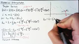
Let’s begin with finite difference methods. These techniques allow us to approximate derivatives using discrete data points. Can anyone tell me about the three types of finite difference methods?

There’s the forward difference, backward difference, and central difference!
Exactly! The forward difference uses the value at the current point and a point ahead. Can anyone express that mathematically?

It’s f’(x) ≈ (f(x+h) - f(x)) / h.
Well done! Now, what about the backward difference?

That's f’(x) ≈ (f(x) - f(x-h)) / h.
Great! And the central difference method is the most accurate. Why do you think that is?

It uses points on both sides of the target point, which gives a better approximation!
Exactly! Remember, the central difference error is O(h²), which is better than the linear error in forward or backward methods. Let's summarize: finite differences help us estimate derivatives. We have forward, backward, and central as key approaches.
Newton-Cotes Formulas
🔒 Unlock Audio Lesson
Sign up and enroll to listen to this audio lesson

Now let’s shift gears to Newton-Cotes formulas for numerical integration. Who wants to tell me what this involves?
It involves approximating an integral by fitting polynomials to the data points.
Correct! The trapezoidal rule is one of the simplest methods. What do you all think are its pros and cons?
It’s easy to implement, but it might be less accurate with fewer intervals.
Exactly, the error decreases linearly with more points. Now, how does Simpson’s rule improve upon this?
It uses quadratic polynomials instead of linear ones, so it’s generally more accurate.
Great observation! Simpson’s rule has an error of O(h⁴). Remember this when deciding which method to use based on required precision!
Gaussian Quadrature
🔒 Unlock Audio Lesson
Sign up and enroll to listen to this audio lesson
Now let’s dive into Gaussian quadrature, a method for numerical integration that can be very efficient. Who can explain how it works?
It approximates integrals using weighted sums of the function values at specific points called nodes.
Exactly! The nodes are not evenly spaced, which helps optimize the approximation. What do you think the advantage of using Gaussian quadrature is?
It can achieve high accuracy with fewer evaluations compared to Newton-Cotes methods!
Exactly! It’s efficient for smooth functions. Remember this when you face integration problems in practical applications. Summarizing: Gaussian quadrature maximizes accuracy with optimized points.
Choosing a Method
🔒 Unlock Audio Lesson
Sign up and enroll to listen to this audio lesson
Finally, let’s talk about choosing between methods. What key factors should we consider?
We need to think about the required accuracy and the computational resources we have.
Correct! Some methods are more computationally intensive than others. How do you think that influences our choices in a real-world scenario?
If resources are limited, we might prefer simpler methods, even if they're less accurate.
Spot on! Understanding these trade-offs is crucial in applying numerical methods effectively. Let’s recap: choose based on accuracy needs and available resources.
Introduction & Overview
Read summaries of the section's main ideas at different levels of detail.
Quick Overview
Standard
In this section, we summarize essential concepts in numerical differentiation and integration. Key topics include finite difference methods for approximating derivatives, Newton-Cotes formulas for integration, and Gaussian quadrature for achieving high accuracy in numerical integration. Understanding these methods is crucial in the fields of engineering, physics, and data analysis.
Detailed
Summary of Key Concepts
This section encapsulates the critical techniques and methods in numerical differentiation and numerical integration as discussed throughout the chapter. The main points include:
- Finite Difference Methods: These are used to approximate derivatives based on discrete data points and include:
- Forward Difference: Uses current and future values.
- Backward Difference: Uses current and past values.
- Central Difference: Employs values from both sides for better accuracy.
- Newton-Cotes Formulas: This family of integration methods includes:
- Trapezoidal Rule: Simple, linear interpolation between data points.
- Simpson’s Rule: Quadratic interpolation providing higher accuracy.
- Higher-order formulas for refined approximations.
- Gaussian Quadrature: A highly efficient integration method that utilizes strategically chosen points and weights to minimize error and maximize accuracy with fewer function evaluations.
- Choosing a Method: The selection of the appropriate technique depends on the specific problem, required accuracy, and available computational resources. Understanding these methods enhances the ability to tackle real-world problems effectively.
Youtube Videos

Audio Book
Dive deep into the subject with an immersive audiobook experience.
Finite Difference Methods
Chapter 1 of 4
🔒 Unlock Audio Chapter
Sign up and enroll to access the full audio experience
Chapter Content
● Finite Difference Methods: Used for approximating derivatives of functions based on discrete points.
Detailed Explanation
Finite Difference Methods are numerical techniques used to estimate the derivative of a function, which represents how a function changes as its input changes. These methods rely on discrete data points rather than continuous functions. By taking the difference between function values at specific points and dividing by the distance between those points (the step size), we can approximate the derivative. Different approaches within finite difference methods include forward difference, backward difference, and central difference, each with varying levels of accuracy and application contexts.
Examples & Analogies
Imagine you are trying to determine the speed of a car at different times based on data you collect every few seconds. By calculating the difference in distance over the difference in time at these intervals, you can estimate how fast the car is going. This is similar to how finite difference methods work with function values to estimate derivatives.
Newton-Cotes Formulas
Chapter 2 of 4
🔒 Unlock Audio Chapter
Sign up and enroll to access the full audio experience
Chapter Content
● Newton-Cotes Formulas: A family of methods for numerical integration, including the trapezoidal rule, Simpson’s rule, and higher-order formulas.
Detailed Explanation
Newton-Cotes Formulas are a set of techniques used for numerical integration. They work by approximating the area under a curve by using polynomials to interpolate the function's values at a given set of discrete points. The trapezoidal rule uses straight line segments to estimate the area, while Simpson’s rule employs parabolic segments to provide a more accurate approximation. As the number of points increases, the accuracy of these formulas improves, making them essential for calculating integrals when an analytic solution is impractical.
Examples & Analogies
Consider trying to find the area of an irregularly shaped plot of land. Instead of measuring the entire area directly, you could divide it into smaller, manageable sections, such as rectangles (trapezoidal rule) or curved sections (Simpson's rule), calculate the area of each section, and then sum them up. This approach mirrors how Newton-Cotes formulas estimate areas under curves.
Gaussian Quadrature
Chapter 3 of 4
🔒 Unlock Audio Chapter
Sign up and enroll to access the full audio experience
Chapter Content
● Gaussian Quadrature: A highly accurate integration method that uses optimized points (nodes) and weights to achieve precision with fewer function evaluations.
Detailed Explanation
Gaussian Quadrature is a sophisticated numerical integration method that aims to achieve high accuracy by selecting specific points, known as nodes, and assigning weights to them. Unlike simpler methods that use evenly spaced intervals, Gaussian Quadrature utilizes strategically chosen non-uniform points, based on the roots of orthogonal polynomials. This allows it to approximate the integral of a function more effectively, producing highly accurate results with fewer function evaluations.
Examples & Analogies
Think about a group of friends trying to decide on a movie to watch. Instead of each person suggesting any random film, they agree to focus on a few well-reviewed films that most people liked. By narrowing down their focus to just a few options, they can make a well-informed choice more efficiently. Similarly, Gaussian Quadrature targets specific points to maximize accuracy in estimating integrals while reducing the need for multiple calculations.
Choosing a Method
Chapter 4 of 4
🔒 Unlock Audio Chapter
Sign up and enroll to access the full audio experience
Chapter Content
● Choosing a Method: The choice of method depends on the problem, required accuracy, and available computational resources.
Detailed Explanation
When faced with numerical differentiation or integration, it is essential to choose the right method based on various factors. These include the nature of the problem, the required level of accuracy, and the computational resources available. For example, simpler methods like the trapezoidal rule may be sufficient for straightforward problems, while more complex situations requiring higher precision may benefit from Gaussian Quadrature. Beginners might start with basic methods and gradually move towards more advanced techniques as their understanding deepens.
Examples & Analogies
Imagine you are cooking a meal. If you're making a simple salad, a basic knife might be sufficient, but for intricate garnishes or precision cuts, you would reach for more specialized kitchen tools. Similarly, when tackling numerical problems, the chosen method should align with the level of complexity and accuracy you need.
Key Concepts
-
Finite Difference Methods: Techniques for approximating derivatives using discrete data points.
-
Newton-Cotes Formulas: A family of numerical integration methods using polynomial interpolation.
-
Gaussian Quadrature: A method that maximizes accuracy using optimally chosen integration points.
-
Choosing a Numerical Method: The decision on which method to use is influenced by required accuracy and computational resources.
Examples & Applications
Example of the forward difference method to approximate the derivative of a function at a specific point.
Demonstration of the trapezoidal rule applied to calculate the area under a curve using a set of discrete points.
Memory Aids
Interactive tools to help you remember key concepts
Rhymes
Forward leaps a step ahead, Backward looks back instead. Central uses both to find, The derivative that's kind!
Stories
Once a wizard named Newton needed to find the treasure's buried location. He had three magic keys: Forward, Backward, and Central, each unlocking different parts of the map of derivatives. The smarter he got, long lost treasures revealed with good polynomial fits!
Memory Tools
Think 'GNC' - Gaussian, Newton-Cotes, Central: three methods to numerically integrate and differentiate.
Acronyms
NICE
Newton-Cotes for Integration
Central for accuracy
and Finite Differences for Derivatives.
Flash Cards
Glossary
- Finite Difference Methods
Techniques used to approximate derivatives of functions based on discrete data points.
- NewtonCotes Formulas
A family of methods for numerical integration that interpolate the integrand using polynomials.
- Gaussian Quadrature
A numerical integration method that utilizes strategically chosen points and weights to maximize accuracy.
- Trapezoidal Rule
A first-order Newton-Cotes formula that approximates the integral using linear interpolation between adjacent points.
- Simpson's Rule
A second-order Newton-Cotes formula that approximates the integral using quadratic polynomials.
- Error in Numerical Methods
The deviation of the approximation from the exact value, often expressed in terms of the step size 'h.'
Reference links
Supplementary resources to enhance your learning experience.