Basic Concept of Finite Difference Methods
Enroll to start learning
You’ve not yet enrolled in this course. Please enroll for free to listen to audio lessons, classroom podcasts and take practice test.
Interactive Audio Lesson
Listen to a student-teacher conversation explaining the topic in a relatable way.
Discretizing the Domain
🔒 Unlock Audio Lesson
Sign up and enroll to listen to this audio lesson

Let's start by talking about how we discretize the domain when using the Finite Difference Method. We take a continuous interval, like [a, b], and break it down into discrete points. Can anyone tell me what those points might be named?

Are they named x0, x1, and so on?

Exactly! These are the grid points where we will approximate the function values. For a 1D problem, we would have points such as x0, x1, ..., xn. Why do we do this?

To make the continuous function manageable for computation?

Absolutely! We can compute approximate values at these discrete points instead of dealing with an infinite number of calculations. Now, what’s the next step after discretizing?

We need to approximate the derivatives!

Correct! This takes us to our next topic.
Approximating Derivatives
🔒 Unlock Audio Lesson
Sign up and enroll to listen to this audio lesson

Now, once we have our grid, we need to approximate the derivatives in our PDE. There are different methods. Let's start with the forward difference method. Can someone explain what that looks like?

It's like using the next point to estimate the slope?

Right! We can express that as: df/dx ≈ (f(x + h) - f(x)) / h. Can someone tell me how this is different from the backward difference?

The backward difference uses the point before instead of after.

Correct! The formula is: df/dx ≈ (f(x) - f(x - h)) / h. And then we also have the central difference. Student_2, can you remind us how that one works?

Yeah! It averages the slopes from the two surrounding points, so it's more accurate.

Exactly! This method is: df/dx ≈ (f(x + h) - f(x - h)) / (2h). All these approximations give us a way to translate our PDE into algebraic equations!
Applying Finite Differences
🔒 Unlock Audio Lesson
Sign up and enroll to listen to this audio lesson

Let's apply what we've discussed. If we take the heat equation, which is a common PDE, how do we apply our finite difference approximations?

We replace the derivatives in the equation with our finite difference approximations?

Correct! So if we take the time derivative as df/dt ≈ (u_i^{n+1} - u_i^n) / Δt, and the spatial second derivative as df/dx^2 ≈ (u_{i+1}^n - 2u_i^n + u_{i-1}^n) / (Δx^2), how do we rearrange these into a usable form?

We can express u_i^{n+1} using those approximations, right?

Exactly right! Each approximation leads to the iterative solution for time steps in the heat equation. That’s how we implement these methods practically.
Advantages and Disadvantages of FDM
🔒 Unlock Audio Lesson
Sign up and enroll to listen to this audio lesson

Finally, let's discuss some strengths and weaknesses of FDM. How would you describe its advantages?

It's simple to implement and effective for regular grids.

Yes! But what about its disadvantages? Student_1?

It struggles with complex geometries and can become less accurate.

Spot on! It's crucial to know both sides when choosing a method to tackle PDEs effectively.
Summary and Reflection
🔒 Unlock Audio Lesson
Sign up and enroll to listen to this audio lesson

As we wrap up, can anyone summarize what we've learned about Finite Difference Methods?

We learned that FDM discretizes the domain into points and approximates derivatives using methods like forward, backward, and central differences.

Absolutely! And what do we conclude about its implementation?

It's useful, but we need to carefully consider its limitations.

Great summary! Remember, while FDM is powerful, the nature of your problem is crucial in deciding whether it's the right choice.
Introduction & Overview
Read summaries of the section's main ideas at different levels of detail.
Quick Overview
Standard
Finite Difference Methods are widely used numerical techniques that approximate the solutions of PDEs by discretizing the domain into a mesh and using finite differences to approximate derivatives. Key approaches are the forward, backward, and central difference methods.
Detailed
Detailed Summary of the Basic Concept of Finite Difference Methods
Finite Difference Methods (FDM) provide a systematic approach for solving partial differential equations (PDEs) by discretizing the equations and the domain of the problem into a finite grid of points. The process involves two main steps:
- Discretizing the Domain: The continuous domain is broken down into a grid where values are computed at specific points. In a 1D case, this involves defining points such as x0, x1, ..., xn within the interval [a, b].
- Approximating Derivatives: Different methods can be employed for approximating derivatives in the PDE:
- Forward Difference: Approximates the derivative using values at the current and next grid point.
- Backward Difference: Uses values at the current and previous grid point.
- Central Difference: Combines information from both sides of the current point for better accuracy.
These approximations transform the PDE into a system of algebraic equations that can be more readily solved using computational techniques. Overall, FDM is simple to implement, making it a popular choice for routine problems in computational mathematics but may struggle with complex geometries.
Youtube Videos


Audio Book
Dive deep into the subject with an immersive audiobook experience.
Discretizing the Domain
Chapter 1 of 2
🔒 Unlock Audio Chapter
Sign up and enroll to access the full audio experience
Chapter Content
The domain is discretized into a grid or mesh, where the continuous variables are approximated by values at specific grid points. For example, for a 1D problem, the domain [a,b] is discretized into points x0, x1, x2,…,x_n.
Detailed Explanation
Discretization is the process of breaking down a continuous domain (which can be thought of as a line or area) into smaller, manageable pieces. This is done by creating a grid or mesh that marks specific points where calculations will take place. In a one-dimensional scenario, if you have a line segment from point 'a' to 'b', you would choose points at regular intervals, labeling them as x0, x1, x2, and so on. Each of these points will represent a specific value of the variable you're interested in, like temperature or pressure.
Examples & Analogies
Imagine you're measuring the temperature of a long metal rod. Instead of measuring the temperature at every single point (which would be impossible and time-consuming), you might decide to measure it at set distances—like every inch along the rod. Each of those measurement points is akin to the discretized grid points you've established.
Approximating Derivatives
Chapter 2 of 2
🔒 Unlock Audio Chapter
Sign up and enroll to access the full audio experience
Chapter Content
The partial derivatives in the PDE are approximated by finite differences. For example:
- Forward Difference:
\( \frac{df}{dx} \approx \frac{f(x+h) - f(x)}{h} \)
- Backward Difference:
\( \frac{df}{dx} \approx \frac{f(x) - f(x-h)}{h} \)
- Central Difference:
\( \frac{df}{dx} \approx \frac{f(x+h) - f(x-h)}{2h} \)
Detailed Explanation
To solve a PDE using finite difference methods, we need to approximate derivatives (which measure how a function changes) with differences between values at discrete points. There are three common types of finite difference approximations:
- Forward Difference - This calculates the change at a point by looking at its value and the value right after it. It's like asking how much the temperature increases from today to tomorrow.
- Backward Difference - This does the opposite, looking at a point and the one right before it, which is like asking how much the temperature decreased from yesterday to today.
- Central Difference - This takes into account both the point before and after, giving a more accurate measure of how a value changes at a specific point. It's like averaging the temperatures before and after today to see how they compare.
By using these approximations, we convert the continuous derivatives in our equations into discrete forms that are easier to solve.
Examples & Analogies
Think about a speedometer in a car. If you want to know how fast you're going, you could look at your position now and in a few seconds (forward difference) or look at your position now and a few seconds ago (backward difference). The central difference is like looking at your car's position halfway between those two moments. By calculating these differences, you can estimate your speed at that moment, which is similar to finding a derivative.
Key Concepts
-
Discretization: Breaking down a continuous domain into discrete points for numerical approximation.
-
Approximating derivatives: Using various methods (forward, backward, central) to approximate derivatives in the PDE.
-
Algebraic equations: The transformed PDEs become solvable algebraic equations using numerical methods.
Examples & Applications
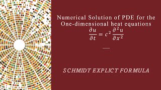
Discretizing the domain in a one-dimensional heat equation where points are defined at intervals to simulate temperature changes over time.
Using a central difference to approximate the second derivative of temperature in a heat transfer problem to create an iterative solution.
Memory Aids
Interactive tools to help you remember key concepts
Rhymes
When the domain's too vast, divide it fast, FDM's design will make it last.
Stories
Imagine you’re a teacher trying to explain a long lesson but can only do so in class periods. You break it into sections, teaching small parts until the students grasp the whole. That's how discretizing helps in FDM!
Memory Tools
Remember 'FBS' for derivative methods: Forward, Backward, and Central.
Acronyms
FDM - Finite Difference Method
Picture it like 'Fast Data Management' for equations!
Flash Cards
Glossary
- Finite Difference Method (FDM)
A numerical technique for approximating solutions to differential equations by discretizing the equations and the domain.
- Discretization
The process of breaking down a continuous domain into a finite number of discrete points.
- Forward Difference
An approximation of a derivative using the function value at the current and next point.
- Backward Difference
An approximation of a derivative using the function value at the current and the previous point.
- Central Difference
An approximation that uses the average of the function values on both sides of a point.
Reference links
Supplementary resources to enhance your learning experience.
