
Numerical Solutions of Partial Differential Equations
Enroll to start learning
You’ve not yet enrolled in this course. Please enroll for free to listen to audio lessons, classroom podcasts and take practice test.
Interactive Audio Lesson
Listen to a student-teacher conversation explaining the topic in a relatable way.
Introduction to Partial Differential Equations (PDEs)
🔒 Unlock Audio Lesson
Sign up and enroll to listen to this audio lesson

Today, we'll explore Partial Differential Equations or PDEs. Can anyone tell me what makes these equations distinct?

PDEs involve functions of several variables and their derivatives, unlike ordinary differential equations.
Exactly! They are pivotal in modeling real-world problems like heat conduction and fluid flow. Why do you think we might not always find analytical solutions for these equations?

Because real-world problems often have complex boundaries or conditions!
Great point! This limitation is where numerical methods come into play. They allow us to obtain approximate solutions effectively.
Finite Difference Methods (FDM)
🔒 Unlock Audio Lesson
Sign up and enroll to listen to this audio lesson

Let’s discuss Finite Difference Methods or FDM. Can someone explain what we mean by 'discretizing the domain'?

It means dividing the continuous domain into a grid with specific points.
Correct! Now, how do we handle derivatives in FDM?

We use finite differences like forward, backward, and central differences!
Well done! Remembering these types can help you in problem-solving. Let's look at an example where we solve the heat equation using this method.
Example of Solving the 1D Heat Equation Using FDM
🔒 Unlock Audio Lesson
Sign up and enroll to listen to this audio lesson
For the 1D heat equation, what initial steps do we take to begin discretization?
We divide the spatial interval into N points and define the time steps.
That's right. And when we apply finite difference approximations, what does the relationship look like?
We substitute our finite differences into the equation, simplifying it to calculate iteratively.
Perfect! This iterative approach allows us to approach the solution effectively.
Finite Element Methods (FEM)
🔒 Unlock Audio Lesson
Sign up and enroll to listen to this audio lesson
Now let’s shift gears to Finite Element Methods, or FEM. What are some advantages of using FEM over FDM?
FEM handles complex geometries and nonlinear problems better than FDM.
Exactly! FEM gives us flexibility with variable geometries. Can anyone summarize the key steps involved in FEM?
We discretize the domain into elements, choose shape functions, formulate the weak form, and assemble the system.
Great summary! Remember these steps when applying FEM in complicated scenarios.
Comparative Overview: FDM vs FEM
🔒 Unlock Audio Lesson
Sign up and enroll to listen to this audio lesson
Finally, let's compare FDM and FEM. What are the main differences?
FDM is simpler and works best on uniform grids, while FEM is for complex shapes and nonlinear issues.
But FEM is also computationally more expensive.
Exactly right! It’s essential to choose the right method based on the problem at hand.
So if we have a simple problem, we can stick with FDM, but for complex cases, we should use FEM.
Perfect summary! Understanding these differences makes you better equipped for solving PDEs.
Introduction & Overview
Read summaries of the section's main ideas at different levels of detail.
Quick Overview
Standard
Numerical solutions of Partial Differential Equations (PDEs) are essential for modeling complex phenomena in simulations. This section introduces two key numerical techniques: Finite Difference Methods (FDM), which are simple and effective for uniform grids, and Finite Element Methods (FEM), which are more flexible for complex geometries and multi-physics problems.
Detailed
Numerical Solutions of Partial Differential Equations
This section details the numerical approaches used to solve Partial Differential Equations (PDEs), which are prevalent in modeling physical systems such as heat transfer, fluid dynamics, and electromagnetic fields. Analytical solutions are often impractical due to complex boundary conditions or geometries, making numerical methods necessary.
Key Methods Discussed
Finite Difference Methods (FDM)
FDM involves discretizing the problem domain and approximating the derivatives using finite differences.
Basic Concepts:
- Discretizing the Domain: The continuous domain is converted into a grid of discrete points.
- Approximating Derivatives: Different finite difference approaches (forward, backward, central) are employed to estimate derivatives in PDEs.
Practical Application: The Heat Equation
An example shows how to solve the 1D heat equation using FDM, demonstrating the discretization of both spatial and time domains followed by applying the finite difference approximations.
Advantages and Disadvantages of FDM
- Advantages: Simplicity and effectiveness for uniform grids.
- Disadvantages: Limited accuracy for complex shapes and geometries.
Finite Element Methods (FEM)
FEM is discussed as a more sophisticated method suitable for complex geometries, nonlinear problems, and multiphysics applications.
Core Steps:
- Discretization: The domain is partitioned into elements, creating a mesh.
- Approximation Functions: Solutions are approximated using shape functions defined on elements.
- Weak Formulation: The governed PDE is transformed into a weak form, easing the computation process.
- Global Equation Assembly: Integrates contributions from all elements to form a system of equations.
Advantages and Disadvantages of FEM
- Advantages: Flexibility to handle complexities and accurate representations.
- Disadvantages: Higher computational cost and the need for careful meshing.
In summary, FDM is suitable for simpler problems, while FEM is necessary for more complex simulations, particularly in multiphysics scenarios.
Youtube Videos
Audio Book
Dive deep into the subject with an immersive audiobook experience.
Introduction to Partial Differential Equations (PDEs)
Chapter 1 of 5
🔒 Unlock Audio Chapter
Sign up and enroll to access the full audio experience
Chapter Content
Partial Differential Equations (PDEs) are equations that involve functions of several variables and their partial derivatives. PDEs are used to model many physical phenomena, such as heat conduction, fluid dynamics, and electromagnetic fields. Solving PDEs analytically is often impossible for real-world problems, especially when boundary conditions or complex geometries are involved. Numerical methods provide approximate solutions to PDEs by discretizing the problem and solving it using computational techniques. In this chapter, we will focus on two popular numerical methods for solving PDEs: Finite Difference Methods (FDM) and Finite Element Methods (FEM).
Detailed Explanation
Partial Differential Equations (PDEs) are important in mathematics and physics because they help describe how physical quantities change with respect to each other. For instance, they can represent the distribution of heat in an object or the motion of fluid. However, these equations can become highly complicated, making them difficult to solve precisely, especially when the systems involved have complex shapes or specific boundaries. This is why we turn to numerical methods, which allow us to get approximate solutions by breaking down these complex problems into smaller, manageable pieces. In this section, we will explore two well-known techniques: Finite Difference Methods (FDM) and Finite Element Methods (FEM).
Examples & Analogies
Imagine baking a cake. While there are many precise ingredients and steps needed to make the perfect cake (analogous to solving PDEs analytically), often we have to adjust the recipe based on what we have at hand (like numerical methods). Sometimes you might decide to estimate the baking temperature or time, which can be viewed as numerical approximations to the perfect cake recipe — and similarly, numerical methods help us approximate solutions where exact answers are hard to get.
Finite Difference Methods (FDM)
Chapter 2 of 5
🔒 Unlock Audio Chapter
Sign up and enroll to access the full audio experience
Chapter Content
Finite Difference Methods (FDM) are among the simplest and most widely used numerical methods for solving PDEs. They involve discretizing the domain and approximating the derivatives in the PDE using finite differences. This transforms the PDE into a system of algebraic equations that can be solved using standard numerical techniques.
Detailed Explanation
Finite Difference Methods provide a framework for approximating solutions to PDEs. The fundamental idea is to replace the continuous variables with discrete points, creating a grid or mesh that represents the domain under consideration. We then use finite differences to approximate the derivatives specified in the PDE, replacing infinitesimal changes with finite steps. This process allows us to reformulate the PDE into linear algebraic equations, which can be solved using computational techniques that are widely available and easy to implement.
Examples & Analogies
Think of someone trying to climb a mountain by taking steps rather than walking continuously. If they take steps of set height (like finite differences), they can still reach the top but might miss nuances and smaller details of the mountain's path. Similarly, FDM takes finite steps to approach solutions to PDEs, making it manageable even when the exact slope or path is complex.
Basic Concept of Finite Difference Methods
Chapter 3 of 5
🔒 Unlock Audio Chapter
Sign up and enroll to access the full audio experience
Chapter Content
- Discretizing the Domain:
- The domain is discretized into a grid or mesh, where the continuous variables are approximated by values at specific grid points. For example, for a 1D problem, the domain [a,b] is discretized into points x0,x1,x2,…,xn.
- Approximating Derivatives:
- The partial derivatives in the PDE are approximated by finite differences. For example:
- Forward Difference: df/dx ≈ (f(x+h)−f(x))/h
- Backward Difference: df/dx ≈ (f(x)−f(x−h))/h
- Central Difference: df/dx ≈ (f(x+h)−f(x−h))/(2h)
Detailed Explanation
The first step in applying FDM is to discretize the problem’s domain. This means dividing the domain into a series of discrete points, allowing for the approximation of continuous functions. In a simple 1D case, you might choose specific locations along a line to evaluate the function. Once you have these points, the next step is to approximate derivatives at these points using finite differences. This can take the form of forward, backward, or central differencing, each of which estimates the derivative based on function values from neighboring points. This process converts the PDE into a form that can be solved as a system of equations, making it feasible with numerical techniques.
Examples & Analogies
Imagine you're reporting the temperature along a road at certain points instead of measuring it continuously. By using a thermometer at specific locations (discretizing), you can get readings (approximations) for each point along the road. You might then calculate the change in temperature using nearby readings. This method helps ensure you get a comprehensive picture of temperature changes without having to measure continuously.
Example: Solving Heat Equation Using FDM
Chapter 4 of 5
🔒 Unlock Audio Chapter
Sign up and enroll to access the full audio experience
Chapter Content
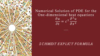
Consider the 1D heat equation: ∂u/∂t=α∂²u/∂x² with initial condition u(x,0)=u0(x) and boundary conditions u(0,t)=uL and u(L,t)=uR.
1. Discretizing the spatial domain: Divide the spatial interval [0,L] into N equally spaced points with spacing Δx=L/N.
2. Discretizing the time domain: Divide the time interval into steps Δt, so the solution is approximated at time points tn=nΔt.
3. Applying the finite difference approximation:
- The spatial second derivative is approximated using the central difference: ∂²u/∂x² ≈ (ui+1n−2uin+ui−1n)/(Δx)²
- The time derivative is approximated using the forward difference: ∂u/∂t ≈ (uin+1−uin)/Δt
4. Substituting these into the heat equation, we get: uin+1−uin/Δt=α(ui+1n−2uin+ui−1n)/(Δx)²
5. Rearranging: uin+1=uin+αΔt/Δx²(ui+1n−2uin+ui−1n). This equation can be solved iteratively for each time step.
Detailed Explanation
Let's apply FDM to solve the heat equation, which describes how heat evolves over time in a one-dimensional rod. First, we identify our spatial and temporal domains. The rod is divided into N equally spaced points, allowing us to measure temperature at each point at different times. Next, we break the time into intervals, at which we want to evaluate the temperature. By applying finite difference rules for both space and time, we can formulate a new equation that expresses how temperature changes over time based on spatial temperatures. This iterative equation allows us to calculate the temperature at the next time step using known values from the current step.
Examples & Analogies
Think of cooking a pot of soup. You want to know how the temperature changes as you cook it. Instead of checking the temperature at every millisecond, you can check it at specific intervals (e.g., every minute). You can then use the temperature from adjacent minutes to estimate its future temperature. Each checking allows you to predict the next state of your soup's temperature, much like how we predict heat changes using the iterative method in FDM.
Advantages and Disadvantages of FDM
Chapter 5 of 5
🔒 Unlock Audio Chapter
Sign up and enroll to access the full audio experience
Chapter Content
Advantages:
- Simple to implement and widely used.
- Effective for problems with uniform grids and simple geometries.
Disadvantages:
- Less accurate for complex geometries or problems with irregular boundaries.
- Requires grid refinement for higher accuracy, leading to higher computational costs.
Detailed Explanation
Finite Difference Methods are praised for their simplicity and ease of implementation, making them a go-to choice for many problems involving PDEs. They work exceptionally well on uniform grids and for straightforward geometrical setups, where the approximation can be reasonably accurate without extensive adjustments. However, the effectiveness can diminish when faced with irregular boundaries or complex geometries. In such cases, obtaining high accuracy may necessitate refining the mesh, which increases computational demands, both in terms of processing power and time.
Examples & Analogies
Consider drawing a straight line versus a wavy line. The straight line is easy to draw and requires a simple, straightforward approach (like FDM with uniform grids). However, when you want to draw the wavy line, you might need a more detailed strategy and additional time to capture each peak and trough (similar to refining your grid for accuracy). What is simple becomes complicated very quickly!
Key Concepts
-
Partial Differential Equations (PDEs): Equations involving functions of multiple variables.
-
Finite Difference Methods (FDM): A straightforward numerical technique for PDEs.
-
Finite Element Methods (FEM): An advanced methodology useful for complex geometries.
Examples & Applications
The heat equation can be solved using finite difference methods by approximating the temperature values on a grid over time.
The Poisson equation can be addressed using Finite Element Methods to handle irregular domains effectively.
Memory Aids
Interactive tools to help you remember key concepts
Rhymes
FDM, simple to begin, just find the points and let it spin. FEM, flexible like a gem, solving shapes with clever stems.
Stories
Imagine a town with roads (FDM), straight and simple, but to build a castle (FEM), you need to know where each brick goes.
Memory Tools
For finite elements, think 'Mesh, Shape, Form, Assemble' - MSAF.
Acronyms
FEM = Find, Every, Middle point
think about locating points in complex shapes!
Flash Cards
Glossary
- Partial Differential Equations (PDEs)
Equations that involve functions of several variables and their partial derivatives.
- Finite Difference Methods (FDM)
A numerical approach that approximates derivatives by discretizing the domain.
- Finite Element Methods (FEM)
A numerical technique that divides a complex problem into smaller, simpler parts or elements.
- Discretization
The process of breaking down continuous functions or equations into discrete form.
- Mesh
The collection of finite elements used in FEM to approximate solutions.
- Weak Form
The formulation of a PDE that reduces the order of derivatives to simplify the problem.
Reference links
Supplementary resources to enhance your learning experience.