
General Time-Domain Steps
Enroll to start learning
You’ve not yet enrolled in this course. Please enroll for free to listen to audio lessons, classroom podcasts and take practice test.
Interactive Audio Lesson
Listen to a student-teacher conversation explaining the topic in a relatable way.
Writing the System Equation
🔒 Unlock Audio Lesson
Sign up and enroll to listen to this audio lesson

Let's begin by discussing how to write the system equation. This step involves using physical laws like Kirchhoff’s laws. Who can remind us what Kirchhoff's laws relate to?

They relate to electrical circuits, specifically current and voltage laws.
Exactly! Now, which law do you think we would use to begin writing our system equation?

We would use Kirchhoff’s voltage law to write the voltage equations.
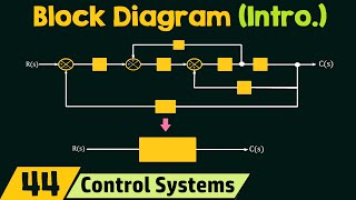
Right! We gather information about loop currents or node voltages to formulate the equations. Remember, a good way to start is by setting up a diagram. This visualization helps us structure the equations efficiently.

So, what's the next step after we've written the system equation?
Great question, Student_3! Next, we take the Laplace transform to simplify our differential equations. This will help us work with algebra instead of calculus.

Why is Laplace transform so useful?
The Laplace transform converts our differential equations into algebraic equations, making them easier to solve. Remember, LAP is often a good acronym to recall: 'Linearize, Algebraize, and Proceed'.
In summary, we write the equation based on physical laws, then apply the Laplace transform to switch to an algebraic format. Let's move on to the next step in our analysis now.
Applying the Laplace Transform
🔒 Unlock Audio Lesson
Sign up and enroll to listen to this audio lesson

Now that we've written our differential equations, let’s talk about the Laplace transform more. Can anyone tell me the general form of the Laplace transform?
I think it's L{f(t)} = F(s) = ∫[0,∞] e^(-st) * f(t) dt.
Correct! This integral helps us transform time-domain functions into the s-domain. It’s essential for handling system equations that are usually complex.
How does this help us with our control systems?
By simplifying those equations. For instance, instead of solving a second-order differential equation, we get to work with a fraction in the s-domain which can be solved with algebra. Can someone give an example of how a simple differential equation is transformed?
If we have a first-order equation like τ dy/dt + y = K, we can transform that to K/s - τY(s).
Excellent! That’s the kind of transformation we will use to simplify our analyses.
To summarize, using the Laplace transform modifies our view of the system, allowing us to solve equations more easily in the s-domain.
Solving for Y(s)
🔒 Unlock Audio Lesson
Sign up and enroll to listen to this audio lesson
At this stage, we need to solve for Y(s), which represents our output signal in the s-domain. What do we require to find Y(s)?
We need the relationship between the input and output, right?
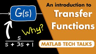
Correct! Finding that relationship often involves manipulating the transfer function of the system. What is the transfer function in basic terms?
It’s the representation of output over input in the frequency domain.
Precisely! By knowing this, we can express Y(s) in terms of R(s), the input. It often looks like Y(s) = G(s) R(s). Can anyone provide an example?
Sure! If we have G(s) = K/(τs + 1) and R(s) = 1/s, then Y(s) would be K/((τs + 1)s).
Exactly! This is a pivotal point because we are just one step away from getting back into the time domain. Who knows what we do next?
We take the inverse Laplace transform!
You’re correct! And to summarize, we derive Y(s) as the output in the s-domain, and it connects to the overall input through the transfer function.
Inverse Laplace Transform
🔒 Unlock Audio Lesson
Sign up and enroll to listen to this audio lesson
Finally, let’s tackle the inverse Laplace transform. Why do we need to do this?
To find out how the system responds over time.
Exactly! The inverse transform allows us to convert our algebraic outcomes back into the time domain. Does anyone recall the common methods we use for finding the inverse?
We can use partial fraction decomposition if it’s a fraction.
Spot on! And we can also use a table of Laplace transforms. For instance, if we see a term that resembles K/(τs + 1), it likely indicates a first-order response.
So once we perform the inverse, we can express y(t). What would y(t) look like for our previous example?
For Y(s) = K/((τs + 1)s), we would find y(t) = K(1 - e^(-t/τ)).
This shows the system approaches K over time, right?
Exactly! In summary, we take Y(s), apply the inverse Laplace transform, and thus obtain the output response of the system in the time domain.
Introduction & Overview
Read summaries of the section's main ideas at different levels of detail.
Quick Overview
Standard
This section describes four essential steps in time-domain analysis. These steps involve deriving the system equation, applying the Laplace transform to obtain a simplified algebraic form, solving for the output in the Laplace domain, and finally conducting the inverse Laplace transform to retrieve the time-domain response.
Detailed
General Time-Domain Steps
In this section, we delve into four crucial steps necessary for time-domain analysis of control systems using block diagrams, which are fundamental in systems engineering. The process begins with defining the system equations through physical laws, such as Kirchhoff’s or Newton's laws. Once the differential equations are established, the next step is to apply the Laplace transform, converting these differential equations into algebraic equations in the complex s-domain, simplifying further calculations. After acquiring the Laplace-transformed equations, we proceed to solve for the output Y(s) in terms of the input, capturing how the input signal transforms through the system. Finally, we utilize the inverse Laplace transform to revert to the time domain, ultimately achieving the system’s time-domain response. This method not only enhances our analytical capabilities but also aids in predicting system behaviors over time.
Youtube Videos
Audio Book
Dive deep into the subject with an immersive audiobook experience.
Step 1 - Write the System Equation
Chapter 1 of 4
🔒 Unlock Audio Chapter
Sign up and enroll to access the full audio experience
Chapter Content
- Write the system equation: Using Kirchhoff’s laws, Newton's laws, or other physical laws to write the differential equation.
Detailed Explanation
In the first step of time-domain analysis, we begin by formulating the system's equation. This involves applying fundamental laws of physics, such as Kirchhoff’s laws for electrical circuits or Newton’s laws for mechanical systems. We derive a differential equation that represents how the system behaves over time in response to inputs. This equation is crucial as it lays the groundwork for the rest of the analysis.
Examples & Analogies
Think of this step as creating a recipe. Just like a recipe lists the ingredients and method to make a dish, writing the system equation is about defining the 'ingredients' (variables and relationships) that describe how our system behaves.
Step 2 - Laplace Transform
Chapter 2 of 4
🔒 Unlock Audio Chapter
Sign up and enroll to access the full audio experience
Chapter Content
- Laplace Transform: Take the Laplace transform of the system equation to obtain the algebraic form in the ss-domain.
Detailed Explanation
Once we have the differential equation from Step 1, we apply the Laplace transform, which is a mathematical technique that converts differential equations into algebraic equations. This transformation simplifies the analysis because algebraic equations are generally easier to solve. In this context, 'ss-domain' refers to the domain of the variable 's', which is a complex frequency variable used in the Laplace transform.
Examples & Analogies
Imagine solving a puzzle. When pieces are scattered, it's difficult to see the whole picture. The Laplace transform gathers the pieces into a clearer structure, allowing us to see and solve the problem more easily.
Step 3 - Solve for Y(s)
Chapter 3 of 4
🔒 Unlock Audio Chapter
Sign up and enroll to access the full audio experience
Chapter Content
- Solve for Y(s): Solve for the Laplace transform of the output in terms of the input.
Detailed Explanation
In the third step, we take the algebraic equation obtained after applying the Laplace transform and rearrange it to isolate Y(s), which represents the Laplace transform of the system's output. This process involves algebraic manipulation, ensuring that we express Y(s) in relation to the input. This output function provides valuable insight into how the system will respond to different inputs in the frequency domain.
Examples & Analogies
Think of this step as deciphering a coded message. Once the puzzle is simplified (like in Step 2), you can more easily identify what message (output) corresponds to each part of the code (input).
Step 4 - Inverse Laplace Transform
Chapter 4 of 4
🔒 Unlock Audio Chapter
Sign up and enroll to access the full audio experience
Chapter Content
- Inverse Laplace Transform: Convert the result back to the time domain to get the system’s time-domain response.
Detailed Explanation
The final step involves applying the inverse Laplace transform to the expression for Y(s) we obtained in Step 3. This operation converts the algebraic solution back into the time domain, allowing us to understand how the system responds over time. The result will be a function of time, typically denoting the output of the system in response to the input.
Examples & Analogies
This step is like baking a cake. The output from the Laplace transform (the transformed recipe) is altered back into the delicious cake we can eat (the time-domain response). Just as the recipe indicates how flavors meld over time, the time-domain response reflects how system outputs evolve.
Key Concepts
-
System Equation: The foundational equation that represents the dynamics of the system based on physical laws.
-
Laplace Transform: A transformation technique that simplifies differential equations into algebraic equations.
-
Y(s): The output in the Laplace domain, which communicates how the system responds to inputs.
-
Inverse Laplace Transform: The process that returns results from the Laplace domain to the time domain, reflecting how a system evolves over time.
Examples & Applications
For a first-order system defined by τ dy/dt + y = K, applying the Laplace transform yields Y(s) = K/(τs + 1).
An example of an inverse Laplace transform is y(t) = K(1 - e^(-t/τ)) for Y(s) = K/((τs + 1)s).
Memory Aids
Interactive tools to help you remember key concepts
Rhymes
Write the laws, take a transform, algebra we will now conform.
Stories
Imagine a story where a system journey begins, first drafting equations from laws of nature’s spins.
Memory Tools
Use L-A-I for the steps of analysis: Law write, Algebra transform, Inverse to time!
Acronyms
R-A-I for Remembering Analysis Steps
Write the equation
Apply Laplace
Inverse back.
Flash Cards
Glossary
- Laplace Transform
A mathematical transformation that converts a function of time into a function of a complex variable, simplifying the analysis of linear time-invariant systems.
- Transfer Function
A mathematical representation of the relationship between the input and output of a linear time-invariant system in the Laplace domain.
- Inverse Laplace Transform
The process of converting a function from the Laplace domain back to the time domain.
- Differential Equation
An equation involving derivatives of a function that describes the relationship between the function and its rates of change.
Reference links
Supplementary resources to enhance your learning experience.