In this chapter, we will walk through a simple design example of an IIR filter (Infinite Impulse Response filter). IIR filters are used widely in signal processing because they can provide efficient solutions to many problems, such as noise removal, frequency shaping, and signal enhancement. We will design a low-pass IIR filter using both the Impulse Invariant Method and the Bilinear Transform Method, which are two common methods of transforming analog filter designs into digital IIR filters. This example will help you understand the practical application of IIR filter design methods and how to implement them in digital signal processing.

We want to design a simple low-pass IIR filter with the following specifications:
● Analog Cutoff Frequency: fc=1 Hz
● Sampling Frequency: fs=10 Hz
● Filter Order: 1st order (to keep the design simple)
Our goal is to design a low-pass filter that attenuates frequencies higher than 1 Hz and passes frequencies below this threshold.

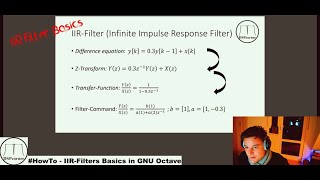
The first step is to design the analog low-pass filter. For this, we can use the standard first-order low-pass filter transfer function in the s-domain (analog): H(s)=Kτs+1 where: ● K is the gain (typically K=1). ● τ is the time constant of the filter, related to the cutoff frequency by τ=12πfc. Given that the cutoff frequency fc=1 Hz, we can calculate the time constant τ: τ=12π⋅1≈0.159 seconds. So, the transfer function of the analog filter is: H(s)=10.159s+1.

The Impulse Invariant Method involves mapping the continuous-time (analog) filter's impulse response to the discrete-time domain. To do this, we apply the transformation s=1−z−1T. ● Sampling Period T=1fs=110=0.1 seconds. ● The impulse response of the analog filter is hanalog(t)=e−tτ. To map the analog filter to the digital domain, we use the formula: H(z)=H(s)∣s=1−z−1T. For our 1st-order low-pass filter, the transfer function in the z-domain is: H(z)=1(1−z−1T⋅0.159+1).

The Bilinear Transform Method maps the entire s-plane to the z-plane using the transformation: s=2T⋅1−z−11+z−1. For a 1st-order low-pass filter, we start with the same analog transfer function: H(s)=1τs+1. Substitute s from the bilinear transform equation: H(z)=1τ(2T⋅1−z−11+z−1)+1. Simplifying this expression results in a new z-domain filter.

Once we have the z-domain transfer function, we can calculate the frequency response of the filter. The frequency response H(ejω) can be found by substituting z=ejω into the transfer function. This provides insight into how the filter behaves in the frequency domain, showing which frequencies are passed and which are attenuated.

Here is a simple Python implementation of the designed IIR low-pass filter using the Bilinear Transform Method with scipy.signal for filter design.

import numpy as np
import scipy.signal as signal
import matplotlib.pyplot as plt
# Design Parameters
fs = 10 # Sampling frequency in Hz
fc = 1 # Cutoff frequency in Hz
tau = 1 / (2 * np.pi * fc) # Time constant
# Design the analog low-pass filter (s-domain)
# H(s) = 1 / (s + 1/tau)
b, a = signal.butter(1, fc, fs=fs, btype='low')
# Frequency Response
w, h = signal.freqz(b, a, fs=fs)
# Plot frequency response
plt.figure()
plt.plot(w, np.abs(h), 'b')
plt.title("Frequency Response of the IIR Low-pass Filter")
plt.xlabel('Frequency [Hz]')
plt.ylabel('Amplitude')
plt.grid(True)
plt.show()

This Python code uses scipy.signal.butter to design a first-order low-pass IIR filter, and it plots the frequency response of the filter. You can modify the fc and fs parameters to adjust the cutoff frequency and sampling rate for different designs.

After obtaining the transfer function, the frequency response of the filter can be analyzed to verify the filter characteristics, such as the cutoff frequency, stopband attenuation, and the shape of the frequency response.
● Cutoff Frequency: The cutoff frequency is where the filter attenuates the signal by 3 dB (half power).
● Passband and Stopband: The filter should allow signals below the cutoff frequency to pass through while attenuating frequencies above the cutoff. For the low-pass filter example, the desired behavior would be:
● Signals below 1 Hz should pass through with minimal attenuation.
● Signals above 1 Hz should be significantly attenuated.

In this chapter, we walked through the design of a simple low-pass IIR filter using the Impulse Invariant and Bilinear Transform Methods. Both methods are widely used for converting analog filter designs to their digital counterparts, each with its advantages:
● The Impulse Invariant Method preserves the time-domain characteristics of the analog filter.
● The Bilinear Transform Method ensures that aliasing is avoided and provides a more accurate digital representation of the analog filter's frequency response.