
Step 2: Apply the Impulse Invariant Method
Interactive Audio Lesson
Listen to a student-teacher conversation explaining the topic in a relatable way.
Introduction to the Impulse Invariant Method
🔒 Unlock Audio Lesson
Sign up and enroll to listen to this audio lesson

Today, we'll explore the Impulse Invariant Method. Can anyone tell me what it means to map an analog filter to a digital filter?

Does it mean converting the analog filter's characteristics into a form we can use in a digital system?
Exactly! The Impulse Invariant Method allows us to preserve the time-domain characteristics of the analog filter. Remember, it keeps the impulse response consistent across domains.

How does the mapping actually work?
Great question! We use the transformation $$s = \frac{1 - z^{-1}}{T}$$ during the process. Who can tell me what $$T$$ represents?

Oh! That's the sampling period, right?
Correct! The sampling period is critical. Remember, $$T = \frac{1}{f_s}$$. Good job! Let's recap: the Impulse Invariant Method focuses on mapping an analog impulse response to a discrete-time representation.
Impulse Response and Time Constant
🔒 Unlock Audio Lesson
Sign up and enroll to listen to this audio lesson

Next, let’s define the impulse response for our low-pass filter. Can anyone recall what the impulse response looks like?
It’s $$h_{analog}(t) = e^{-\frac{t}{\tau}}$$, right?
Correct! And we need to calculate the time constant $$\tau$$ for our analog filter. How do we find it based on the cutoff frequency?

Is it $$\tau = \frac{1}{2\pi f_c}$$?
Exactly! For our case, with a cutoff frequency $$f_c = 1 Hz$$, what does that give us for $$\tau$$?
$$\tau ≈ 0.159$$ seconds!
Brilliant! Now we can express the impulse response as $$h_{analog}(t) = e^{-\frac{t}{0.159}}$$. Let's remember this key concept as we proceed.
Transforming to the Discrete-Time Domain
🔒 Unlock Audio Lesson
Sign up and enroll to listen to this audio lesson
Now, we will apply the transformation to convert the analog filter design into a digital filter. Can anyone recall the equation we use?
It's $$H(z) = H(s) \Bigg|_{s = \frac{1 - z^{-1}}{T}}$$!
Exactly! Now, substituting our values into the equation, let’s begin simplifying. We have $$H(z) = \frac{1}{(0.159 \cdot \frac{1 - z^{-1}}{0.1}) + 1}$$. What should we do next?
We can substitute $$T$$ and simplify further!
Correct! Let's simplify and see what our discrete-time transfer function is. What does it look like?
$$H(z) = \frac{1}{(1.59 - 1.59z^{-1}) + 1}$$.
Excellent! So, we now have our digital filter's representation, reflecting the behavior of the original analog filter.
Significance in Digital Signal Processing
🔒 Unlock Audio Lesson
Sign up and enroll to listen to this audio lesson
Finally, let’s discuss why the Impulse Invariant Method is significant in digital signal processing. Who can share their thoughts?
It allows us to keep the characteristics of the analog filter, right?
Exactly! By preserving time-domain characteristics, it provides a smooth transition into digital systems. What are some applications you think might benefit from this method?
I guess in audio processing for sound restoration or noise reduction?
Good point! Also, in telecommunications and digital media, this method ensures that filters maintain their intended performance across different systems.
It's fascinating how a mathematical approach can impact so many practical areas!
Absolutely! In summary, the Impulse Invariant Method is pivotal in designing effective digital filters while retaining analog characteristics. Always remember its role in enabling efficient digital signal processing.
Introduction & Overview
Read summaries of the section's main ideas at different levels of detail.
Quick Overview
Standard
The Impulse Invariant Method allows the translation of an analog filter's impulse response into the digital domain. It consists of mapping the s-domain transfer function into the z-domain through a specific transformation, thus enabling the analysis and design of digital filters based on their analog counterparts.
Detailed
Step 2: Apply the Impulse Invariant Method
The Impulse Invariant Method is a technique used to transform a continuous-time (analog) filter's impulse response into the discrete-time domain. The success of this method lies in the correct mapping of the s-domain representation to the z-domain, facilitating the analysis and implementation of digital IIR filters. In this context, we begin by determining the analog filter's impulse response, which for our low-pass filter is defined as:
$$h_{analog}(t) = e^{-\frac{t}{\tau}}$$
where $$\tau$$ is the time constant derived from the cutoff frequency. This transformation requires substituting the s-domain variable with $$s = \frac{1 - z^{-1}}{T}$$, where $$T$$ is the sampling period (for our example 0.1 seconds). Combining these parameters, we derive the z-domain transfer function:
$$H(z) = \frac{1}{(0.159 \cdot \frac{1 - z^{-1}}{0.1}) + 1}$$
Upon substituting and simplifying, we arrive at:
$$H(z) = \frac{1}{(1.59 - 1.59z^{-1}) + 1}$$
This digital transfer function retains the behavior of the original analog low-pass filter, thus enabling effective digital signal processing applications.
Youtube Videos

Audio Book
Dive deep into the subject with an immersive audiobook experience.
Introduction to the Impulse Invariant Method
Chapter 1 of 6
🔒 Unlock Audio Chapter
Sign up and enroll to access the full audio experience
Chapter Content
The Impulse Invariant Method involves mapping the continuous-time (analog) filter's impulse response to the discrete-time domain.
Detailed Explanation
The Impulse Invariant Method is a technique used to convert an analog filter into a digital one by focusing on the filter's impulse response. In signal processing, impulse response defines how a system reacts over time to an impulse input. This method preserves the shape of the impulse response, but it does require a sampling process to transition from analog to digital.
Examples & Analogies
Think of this method like creating a digital snapshot of a smooth fade-out of music. If you take pictures at regular intervals of the fade-out, when you play these images in sequence, they recreate the smooth transition in a digital format.
Transformation of Variables
Chapter 2 of 6
🔒 Unlock Audio Chapter
Sign up and enroll to access the full audio experience
Chapter Content
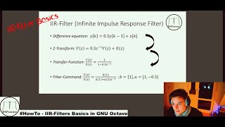
To do this, we apply the transformation s=1−z−1T.
Detailed Explanation
In order to map the analog filter (represented by the variable 's') into the digital domain (represented by the variable 'z'), we use the transformation formula s = (1 - z^(-1)) / T, where 'T' is the sampling period. This transformation plays a crucial role in linking the continuous-time signal with discrete-time systems, allowing the analog filter's behavior to be understood using digital terms.
Examples & Analogies
Imagine translating a book from one language to another while maintaining the original message. The variables 's' and 'z' act as the languages of the filter, and the transformation ensures the message stays the same, just in a different context.
Finding the Sampling Period
Chapter 3 of 6
🔒 Unlock Audio Chapter
Sign up and enroll to access the full audio experience
Chapter Content
Sampling Period T=1/fs=1/10=0.1 seconds.
Detailed Explanation
The sampling period 'T' is the time duration between each sample taken from the continuous signal. In this case, the sampling frequency 'fs' is given as 10 Hz, which means we collect 10 samples every second. This translates to a sampling period of 0.1 seconds, indicating how frequently we sample the signal.
Examples & Analogies
Consider taking photos of a moving car. If you take a photo every 0.1 seconds while the car drives, you will have 10 pictures of it after one second, giving you a comprehensive view of its movement without missing too much detail.
Impulse Response of the Analog Filter
Chapter 4 of 6
🔒 Unlock Audio Chapter
Sign up and enroll to access the full audio experience
Chapter Content
The impulse response of the analog filter is h_analog(t)=e^(−t/τ).
Detailed Explanation
The impulse response represents how the filter responds over time when subjected to a quick pulse (impulse). The given formula, h_analog(t) = e^(-t/τ), shows that the response decays exponentially based on the time constant 'τ.' This decay is integral to predicting how the filter will behave when different signals are applied.
Examples & Analogies
Imagine dropping a pebble into a still pond. The ripples created will slowly fade as they move outward—this fading represents how the impulse response of the filter declines over time, demonstrating its sensitivity to initial impulses.
Mapping the Analog Filter to Digital Domain
Chapter 5 of 6
🔒 Unlock Audio Chapter
Sign up and enroll to access the full audio experience
Chapter Content
To map the analog filter to the digital domain, we use the formula: H(z)=H(s)|_{s=(1−z^{−1})/T}.
Detailed Explanation
Using the transformation we established earlier, we now substitute the 's' variable in our transfer function H(s) with its equivalent in the digital domain. This results in a new function H(z), which characterizes the filter's behavior in the discrete-time framework. This step is crucial for ensuring that the digital filter mirrors the attributes of the original analog filter.
Examples & Analogies
Consider converting a handwritten recipe into a typewritten one. While the content stays the same, the method of presentation changes to a new format. Here, H(z) acts like the typewritten recipe—retaining the original information but transformed for a new purpose.
Final Form of the Transfer Function
Chapter 6 of 6
🔒 Unlock Audio Chapter
Sign up and enroll to access the full audio experience
Chapter Content
For our 1st-order low-pass filter, the transfer function in the z-domain is: H(z)=1(1.59−1.59z−1)+1.
Detailed Explanation
After performing the necessary transformations and substitutions, we establish the discrete-time transfer function for the low-pass filter. It is represented as H(z) = 1 / (1.59 - 1.59z^(-1)) + 1. This equation describes how the filter will process incoming signals in the digital domain, specifically outlining the relationship between the output and input signals.
Examples & Analogies
You can think of this transfer function like a new recipe for a dish you are preparing. After following a certain process (the mathematical transformations), you have a complete formula that helps you replicate a consistent flavor (the desired filter behavior).
Key Concepts
-
Impulse Invariant Method: A method for converting an analog filter's impulse response to a digital filter form.
-
Sampling Period (T): The duration between samples in a discrete-time system.
-
Time Constant (τ): Determines the response speed of the filter, linked to the cutoff frequency.
-
Cutoff Frequency (fc): The frequency at which the output signal is significantly reduced.
Examples & Applications
Example of using the Impulse Invariant Method to design a filter that meets specific cutoff frequency requirements.
Illustration of how the impulse response changes from analog to digital form.
Memory Aids
Interactive tools to help you remember key concepts
Rhymes
To transform an impulse with no haste, into digital that we can taste. The Invariant Method we embrace!
Stories
Imagine a filter taking a leap, from analog waves to digital deep. It keeps its character, never to weep.
Memory Tools
To remember the steps: 'Impulse from s to z, keep T, let it be!'.
Acronyms
TIP
Time domain
Impulse response
Preserved characteristics.
Flash Cards
Glossary
- Impulse Invariant Method
A technique used to map the impulse response of an analog filter into the digital domain.
- Sampling Period (T)
The inverse of the sampling frequency, determining the intervals at which the signal is sampled.
- Time Constant (τ)
A parameter that defines the rate at which the filter responds to changes in the input signal.
- Cutoff Frequency (fc)
The frequency at which the filter begins to attenuate input signals.
- Analog Filter
A filter that processes continuous-time signals.
- Digital Filter
A filter that processes discrete-time signals.
Reference links
Supplementary resources to enhance your learning experience.