
Dispersion Models
Enroll to start learning
You’ve not yet enrolled in this course. Please enroll for free to listen to audio lessons, classroom podcasts and take practice test.
Interactive Audio Lesson
Listen to a student-teacher conversation explaining the topic in a relatable way.
Point Source vs. Area Source
🔒 Unlock Audio Lesson
Sign up and enroll to listen to this audio lesson

Today, we're exploring point sources and area sources in dispersion models. Can anyone tell me what a point source is?

A point source is a fixed location where pollutants are released, like a factory smokestack.
Exactly! And what about area sources?

An area source is a broader emission site, like a landfill that emits pollutants over a larger area.
Great! Remember, the classification can change based on the observational scale. If we zoom out far enough, even the landfill might appear as a point source. This leads us to consider how emissions scale over distances.

So, if I understood correctly, modeling has to adjust according to the scale we are examining?
Absolutely correct! That's the key takeaway. Scale adjustments are crucial in ensuring accurate dispersion estimates.
Additive vs. Non-Additive Contributions
🔒 Unlock Audio Lesson
Sign up and enroll to listen to this audio lesson

Next, let's discuss how multiple sources contribute to pollutant concentrations. What is the assumption about their contributions?

They are usually assumed to be additive, right?
Yes, but that's not always true. Can anyone think of why?
Because the pollutants could interact in the atmosphere and create different concentrations?
Exactly! This means real-life conditions can lead to non-linear interactions, and that's something we have to consider in our models.
So we can't just add everything together without understanding the interactions?
Correct! Understanding the dynamic nature of pollutants helps in developing more accurate models.
Gaussian Dispersion Model
🔒 Unlock Audio Lesson
Sign up and enroll to listen to this audio lesson
Let’s dive into the Gaussian dispersion model. Who can tell me how it's used in environmental monitoring?
It estimates pollutant concentrations based on emission rates and meteorological conditions?
Fantastic! Can you summarize the key factors it takes into account?
Wind speed, emission rate, and dispersion coefficients, like sigma y and sigma z.
Exactly right! These factors combine to provide a steady-state estimate of concentration. What’s the primary benefit of using this model?
It’s a quick method for screening potential pollution impacts.
Spot on! It gives us a preliminary assessment to work from. Remember, it's just the first step in analysis!
Regulatory Models: AERMOD and CALPUFF
🔒 Unlock Audio Lesson
Sign up and enroll to listen to this audio lesson
Finally, we’ll discuss regulatory models like AERMOD and CALPUFF. What distinguishes AERMOD from ISC3?
AERMOD uses more sophisticated meteorological data and does not rely on stability classes.
Correct! And how about CALPUFF?
CALPUFF can handle non-steady state emissions and converts that into a puff-based model.
Exactly! These models are essential for compliance with air quality standards and predicting potential pollutant impacts.
Introduction & Overview
Read summaries of the section's main ideas at different levels of detail.
Quick Overview
Standard
This section delves into the mechanics of dispersion models, emphasizing the Gaussian model and the effects of multiple sources. It explores concepts such as point sources, area sources, and the distinction between steady and unsteady emissions, along with mentioning regulatory models like AERMOD and CALPUFF.
Detailed
Dispersion Models
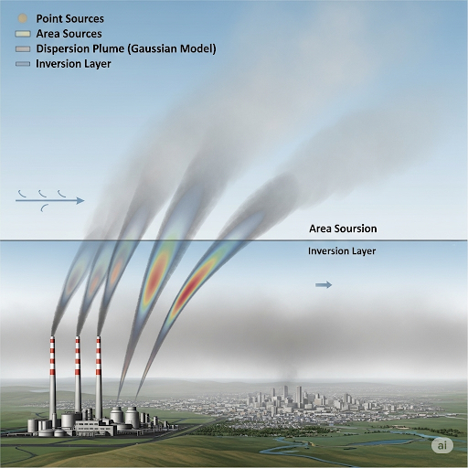
Dispersion models are mathematical tools that analyze how pollutants disperse in the atmosphere from various sources, such as industrial stacks or garbage dumps. In this section, we primarily focus on the Gaussian dispersion model and its application in environmental monitoring.
Key Concepts
- Point Source vs. Area Source: A point source is a single, identifiable pollution source, while an area source encompasses a broader emission source, such as a landfill. Depending on the geographical scale observed, the classification of a source can change from area to point source.
- Additive vs. Non-Additive Contributions: The models often assume that contributions from multiple sources are additive; however, real interactions between pollutants can complicate this. The non-linearity in dispersion can lead to decreased concentrations at receptors due to various mixing effects.
- Gaussian Dispersion Model: Used for quick estimates, this model assumes steady-state conditions and provides basic calculations of concentration levels based on wind speed, emission rates, and dispersion coefficients.
- AERMOD and CALPUFF: These are regulatory models used for air quality analysis, with AERMOD focusing on steady-state emissions while CALPUFF accommodates unsteady-state releases.
Practical Implications
The information gathered from dispersion modeling plays a crucial role in environmental quality assessments and regulatory compliance, particularly in predicting the potential impacts of pollution on public health and ecosystems.
Youtube Videos


Audio Book
Dive deep into the subject with an immersive audiobook experience.
Introduction to Dispersion Models
Chapter 1 of 8
🔒 Unlock Audio Chapter
Sign up and enroll to access the full audio experience
Chapter Content
So last class, we were discussing the application of dispersion models. We will just recap from that little bit.
Detailed Explanation
The lecturer begins by introducing the concept of dispersion models, indicating that this topic was discussed in the previous class. Essentially, dispersion models are used to understand how pollutants move through the air from their source into the surrounding environment. This introduction sets the stage for the deeper exploration of different types of dispersion models and their applications that will follow.
Examples & Analogies
Think of a drop of ink in water. When you drop ink into a glass of water, the ink doesn’t just stay in one place; it spreads out. A dispersion model helps predict how that ink (or in the case of air pollution, a pollutant) will spread out through the environment.
Application of Dispersion Models
Chapter 2 of 8
🔒 Unlock Audio Chapter
Sign up and enroll to access the full audio experience
Chapter Content
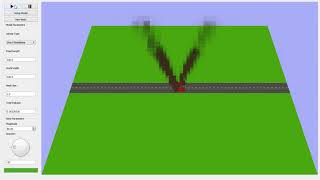
So, one of the applications the way we apply it is superimpose calculation of dispersion models over a given geographical location.
Detailed Explanation
Dispersion models can be applied in practical scenarios by overlaying calculations on specific geographical locations. This means using a model to see how pollutants from a source (like a factory or landfill) will disperse in the air over the surrounding area. The calculations involve understanding three dimensions: x, y, and z coordinates, which represent horizontal and vertical distances in relation to the pollutant source. Analysts must adjust the coordinates based on where different sources are located to estimate their cumulative impact.
Examples & Analogies
Imagine you're a teacher in a classroom and you throw a handful of confetti into the air. The confetti spreads out in different directions and at different heights. A dispersion model helps predict how the confetti, like pollutants, will scatter through the room.
Adjusting Coordinates for Multiple Sources
Chapter 3 of 8
🔒 Unlock Audio Chapter
Sign up and enroll to access the full audio experience
Chapter Content
However, when you are looking at concentrations at a given point is the contribution from different source, then you have to adjust the coordinates accordingly.
Detailed Explanation
When evaluating the concentration of pollutants at a specific point, especially when several sources are present, it requires careful adjustment of coordinates. Each source has its own reference point; if there are multiple sources, their impacts on the concentration must be added while considering their distances and directions. This process can be complex, as different sources can influence the concentration at a measurement point differently.
Examples & Analogies
If you are in a room with multiple air fresheners placed at varying distances, the scent's intensity you perceive will depend on how close each freshener is to you. The closer the freshener, the stronger the scent. Coordinating these distances in a dispersion model works similarly when calculating how pollution from various sources affects air quality.
Additive Contributions and Real-World Implications
Chapter 4 of 8
🔒 Unlock Audio Chapter
Sign up and enroll to access the full audio experience
Chapter Content
So which reference are you taking. So you have to add accordingly okay, where the contribution from different sources is additive, there is no assumption that one source interferes with the other, which is not true in reality.
Detailed Explanation
In the simplistic view of dispersion models, it is assumed that contributions from different sources can be simply added together. This means that the effects of one pollutant source do not interfere with those of another, which simplifies the calculations. However, in reality, pollutants can interact, leading to different behavior than predicted by straightforward addition. Hence, while this assumption makes for easier calculations, it doesn't always reflect the complexity of real-world pollution dynamics.
Examples & Analogies
Consider how two pieces of music playing simultaneously can create a soundscape that's different from the sum of the individual sounds. If you listen to two songs together, they may blend in ways that overpower certain notes or create harmonies, just like how pollutants can react with each other in the environment.
Limitations of Simplistic Dispersion Models
Chapter 5 of 8
🔒 Unlock Audio Chapter
Sign up and enroll to access the full audio experience
Chapter Content
However, when looking at air masses, they do not mix nicely. There will be collision and there will be a local circulation there and all that, all those issues are there, it will neglect all that.
Detailed Explanation
The lecturer points out a significant limitation of basic dispersion models: they don't account for the complexities and dynamics of how air masses behave in reality. In the atmosphere, air flows can collide or create local turbulence, which impacts the dispersion of pollutants. Because of these dynamics, predictions made by basic models may not always match real-world observations, highlighting a critical gap that more advanced models attempt to address.
Examples & Analogies
Imagine a crowded room where people are walking in different directions. While you might predict where a person will end up based solely on their initial position and direction, the actual path they take may change due to collisions with others or obstacles, similar to how air masses interact and complicate dispersion.
Introducing Advanced Dispersion Modeling
Chapter 6 of 8
🔒 Unlock Audio Chapter
Sign up and enroll to access the full audio experience
Chapter Content
However, there are some corrections to that people do, that is a different issue, it is a little more advanced that needs more information about the air mass and all that.
Detailed Explanation
Advanced dispersion modeling techniques take into account the interactions between different air parcels and pollutants. Unlike basic models, these advanced models require comprehensive data about the air mass, including its speed, direction, temperature, and characteristics. They aim to provide a more accurate representation of how pollutants disperse by considering factors like turbulence and local air movement.
Examples & Analogies
Think about a weather forecast that incorporates not only temperature and humidity but also wind patterns and topographical features like mountains and valleys. Such forecasts are much more accurate than simple predictions that only look at one aspect, similar to how advanced models work for air pollution dispersion.
Comparison of Modeling Techniques
Chapter 7 of 8
🔒 Unlock Audio Chapter
Sign up and enroll to access the full audio experience
Chapter Content
The problem is all environmental modeling is which which all depends on the amount of data you have.
Detailed Explanation
The effectiveness of any environmental dispersion model heavily relies on the quality and quantity of the input data. More sophisticated models need extensive meteorological data and information about pollutant characteristics to make reliable predictions. Without adequate data, even the best models may provide inaccurate assessments of the dispersion of pollutants, which can impede effective decision-making in environmental management.
Examples & Analogies
Imagine trying to cook a complicated recipe without knowing the correct measurements for each ingredient. Just as using the wrong amounts can ruin a dish, insufficient or incorrect data can lead to poor predictions in dispersion models.
Modeling in Relation to Weather Forecasting
Chapter 8 of 8
🔒 Unlock Audio Chapter
Sign up and enroll to access the full audio experience
Chapter Content
This becomes like weather forecasting because weather prediction you are predicting wind speed and temperatures and all that.
Detailed Explanation
The lecturer compares dispersion modeling to weather forecasting, emphasizing that both processes involve predicting how specific factors—such as wind speed and temperature—affect behavior over time. Just as weather predictions require accurate information about atmospheric conditions to forecast weather effectively, pollution dispersion models utilize meteorological data to understand how pollutants spread and interact in the environment.
Examples & Analogies
Just like a weather reporter uses radar and other tools to predict rain, a dispersion modeler collects various data points to predict how pollutants spread into the atmosphere, ensuring that we can anticipate and prepare for the consequences.
Key Concepts
-
Point Source vs. Area Source: A point source is a single, identifiable pollution source, while an area source encompasses a broader emission source, such as a landfill. Depending on the geographical scale observed, the classification of a source can change from area to point source.
-
Additive vs. Non-Additive Contributions: The models often assume that contributions from multiple sources are additive; however, real interactions between pollutants can complicate this. The non-linearity in dispersion can lead to decreased concentrations at receptors due to various mixing effects.
-
Gaussian Dispersion Model: Used for quick estimates, this model assumes steady-state conditions and provides basic calculations of concentration levels based on wind speed, emission rates, and dispersion coefficients.
-
AERMOD and CALPUFF: These are regulatory models used for air quality analysis, with AERMOD focusing on steady-state emissions while CALPUFF accommodates unsteady-state releases.
-
-
Practical Implications
-
The information gathered from dispersion modeling plays a crucial role in environmental quality assessments and regulatory compliance, particularly in predicting the potential impacts of pollution on public health and ecosystems.
Examples & Applications
An industrial factory is a point source, while a landfill can be an area source depending on the scale used for modeling.
The Gaussian dispersion model can be applied to estimate the concentration of pollutants emitted from a power plant under steady-state conditions.
Memory Aids
Interactive tools to help you remember key concepts
Rhymes
From factories tall, pollutants fall, in point sources, they stand tall.
Stories
Once upon a time, a factory released smoke into the air, and a nearby landfill spread its waste. The winds danced around them, leading to various concentrations of pollutants, showcasing the importance of understanding different sources.
Memory Tools
P.A.G: Point, Area, Gaussian models - remember the key types of dispersion models.
Acronyms
GREAT
Gaussian
Regulatory
Emissions
Additive
Trends - a reminder of key concepts in dispersion modeling.
Flash Cards
Glossary
- Dispersion Model
A mathematical tool for predicting how pollutants disperse in the atmosphere from a source.
- Point Source
A single, identifiable location where pollutants are emitted.
- Area Source
A broader emission source, such as a landfill, that emits pollutants over a larger area.
- Gaussian Model
A model used to estimate pollutant concentrations based on several variables like wind speed and emission rates.
- AERMOD
A regulatory dispersion model that provides steady-state estimates of air quality.
- CALPUFF
A regulatory dispersion model that addresses non-steady state emissions and uses a puff approach.
Reference links
Supplementary resources to enhance your learning experience.