
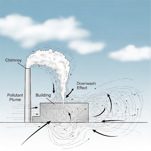
Downwash Effects
Enroll to start learning
You’ve not yet enrolled in this course. Please enroll for free to listen to audio lessons, classroom podcasts and take practice test.
Interactive Audio Lesson
Listen to a student-teacher conversation explaining the topic in a relatable way.
Introduction to Downwash Effects
🔒 Unlock Audio Lesson
Sign up and enroll to listen to this audio lesson

Today, we're discussing downwash effects. Who can tell me what downwash refers to in the context of air dispersion?

Is it when pollutants get pushed downwards by buildings or other structures?
Exactly! Downwash is the downward movement of air caused by obstacles. It plays a significant role in how pollutants disperse.

How do we model these downwash effects?
Good question. We use dispersion models like the Gaussian model, but we must remember that these models often assume additive effects. That means they don't account for the complexities of how air masses mix.

So it's not always straightforward?
Correct! In reality, factors like turbulence and nearby sources create complicated interactions. Let's keep these in mind as we explore further different scenarios of source emissions.
Gaussian Dispersion Model
🔒 Unlock Audio Lesson
Sign up and enroll to listen to this audio lesson

Let’s discuss the Gaussian dispersion model. It’s widely used for predicting pollutant behavior. Can anyone explain how it works?
It predicts how pollutants disperse from a point source by assuming a bell-shaped distribution.
That's right! But what about the assumption of additive contributions? How does this affect our predictions?

It means we might underestimate or overestimate pollution levels because it doesn’t account for interactions between substances.
Exactly! If we have multiple sources, their emissions can interact in non-linear ways, particularly in urban areas.
So, what’s the result of this model’s limitations in real-life scenarios?
Great observation! The results can lead to miscalculations in pollution predictions, which can impact regulations and public health assessments.
Real-World Examples of Downwash Effects
🔒 Unlock Audio Lesson
Sign up and enroll to listen to this audio lesson
Let's connect today’s material to real-world scenarios. Can anyone think of a specific example of downwash effects?
The Perungudi garbage dump you mentioned earlier is a good example. It’s an area source of emissions.
Absolutely! This area has dimensions that can be modeled as an area source rather than a point. As we zoom out, it appears as a point source.
So, depending on the scale of the map we're looking at, our modeling approach changes?
Exactly! Adjusting our model parameters is crucial for accurate predictions in different contexts.
Comparison of AERMOD and CALPUFF
🔒 Unlock Audio Lesson
Sign up and enroll to listen to this audio lesson
Now let’s compare two significant models: AERMOD and CALPUFF. What’s a key difference between them?
I think AERMOD is more steady-state, while CALPUFF uses a puff model for unsteady emissions?
Correct! AERMOD works well for regulatory purposes in steady conditions. CALPUFF is applicable where emissions are not constant.
So both models have their uses, depending on the emission scenario.
Exactly! Knowing which model to apply is essential for appropriate risk assessment and environmental quality monitoring.
Introduction & Overview
Read summaries of the section's main ideas at different levels of detail.
Quick Overview
Standard
This section outlines key concepts related to downwash effects, including how they influence dispersion models. It highlights the limitations of additive assumptions in dispersion modeling, especially in urban environments with multiple emission sources contributing simultaneously.
Detailed
Detailed Summary
In this section, we delve into the concept of downwash effects in dispersion modeling, an essential aspect of environmental quality monitoring. Downwash refers to the downward motion of air and pollutants caused by atmospheric turbulence and obstacles such as buildings or stacks. The interaction between air masses emitted from different sources complicates the prediction of pollutant concentrations, as these emissions often do not mix uniformly.
The session outlines how various dispersion models, such as the Gaussian dispersion model, assume the contribution of each pollutant source is additive; however, this assumption often falls short in real-world scenarios. For instance, downwash from nearby buildings can alter the expected dispersion pattern, leading to localized concentrations that deviate from predictions.
Discussing real-world examples, such as emissions from a point source like a chimney or an area source like a garbage dump, demonstrates how model parameters need adjustments based on scale and spatial considerations. The section also highlights the use of models like AERMOD and CALPUFF, emphasizing their differences and applications in accurately predicting pollution spread in urban settings. Understanding these downwash effects is crucial for effective air quality regulation, as they directly impact public health and environmental policies.
Youtube Videos


Audio Book
Dive deep into the subject with an immersive audiobook experience.
Introduction to Downwash Effects
Chapter 1 of 4
🔒 Unlock Audio Chapter
Sign up and enroll to access the full audio experience
Chapter Content
So, we talked about stacktip downwash, building downwash and all that last time. This is the multiple stacks. So, you have several stacks. All of them contributing to this thing, so it is usually additive, but here you are seeing that it is not just additive, it is slightly lower than N raised to 1.
Detailed Explanation
In this chunk, the concept of downwash effects from multiple stacks is introduced. Downwash refers to the downward movement of contaminated air, often caused by buildings or stacks obstructing the flow of air. It indicates that when collecting air pollution data from multiple sources—like smokestacks—the concentrations from these sources do not add up in a straightforward way. This is because physical interactions and the mixing of air masses can lead to a lower effective concentration reaching the ground than would be predicted by simple addition. Mattes are made complex by the interactions among pollutants, which experience a combined effect that is less than expected.
Examples & Analogies
Imagine pouring several different colored paints into a bucket. If you pour them in directly without mixing, they may seem to blend together, much like how pollutants could mix in the atmosphere. However, if you stir the paints, the colors might swirl together in unexpected ways, creating a new shade that is different from the sum of the individual colors. This is similar to how pollutants interact in the air and why we can't just add their concentrations together.
Experimental Findings on Contribution Factors
Chapter 2 of 4
🔒 Unlock Audio Chapter
Sign up and enroll to access the full audio experience
Chapter Content
The contribution factor by which we multiply centerline concentration from a single stack is found experimentally to be about N raised to 4 by 5. So, the number of stacks is not straight additive, it is lesser than that, which means that there is some loss in the process of doing this.
Detailed Explanation
This chunk discusses the empirical finding that when measuring the impact of multiple emission sources, the resulting concentration at a location does not increase linearly with the number of sources (stacks). Instead, it increases by a factor of N raised to 4/5, indicating that adding more stacks results in diminishing returns regarding their collective impact. This loss can be attributed to physical phenomena such as air mixing and dispersion, which reduce the efficiency of the pollutants reaching a receptor point.
Examples & Analogies
Think of a crowded concert where the sound from multiple speakers (stacks) is supposed to create an immersive experience. If you add more speakers, initially, the sound gets louder, but eventually the sound can become muddled or distorted due to overlapping waves, meaning that not all speakers contribute equally to volume. Thus, even though more speakers are present, the perceived volume might not increase proportionately, similar to pollutant concentrations from multiple stacks.
Understanding Plume Mixing
Chapter 3 of 4
🔒 Unlock Audio Chapter
Sign up and enroll to access the full audio experience
Chapter Content
Generally, when you are talking about plumes, air masses they mix and there are other secondary effects to that, which is still not very clear. In order to quantify them, you have to go and do a fluid mechanic model.
Detailed Explanation
This chunk points out that air pollution plumes from stacks do not behave in a straightforward manner. As they travel, they mix and interact with each other and surrounding air masses. These interactions can create unpredictable behaviors (secondary effects) that complicate the modeling of their dispersion. To accurately predict the behavior of these plumes, advanced fluid mechanics models must be employed, as they can capture the complexities of turbulent flows and their effects on pollutant dispersion.
Examples & Analogies
Consider a pot of boiling soup on the stove. The heat creates convection currents that cause the soup to mix, distributing flavors and temperatures throughout the pot. Similarly, in the atmosphere, warm and cold air can cause pollution to mix and swirl in unpredictable ways, making it more challenging to know exactly where pollutants will go.
Impact of Boundaries on Plume Behavior
Chapter 4 of 4
🔒 Unlock Audio Chapter
Sign up and enroll to access the full audio experience
Chapter Content
Suppose there is what we call a bluff means, this is like either a mountain or a building or something in the path in the y direction. The ground reflection we talked about is a z direction reflection, so there can also be y direction reflection if there is a big building or a big mountain and there is a source.
Detailed Explanation
In environmental modeling, the presence of physical structures like buildings or mountains can significantly alter how a pollutant plume behaves as it travels through the atmosphere. These obstacles can reflect or alter the direction of the plume—what is referred to as 'bluff body effects.' This can lead to concentration peaks in unexpected areas, necessitating the consideration of such structures in dispersion models for accurate predictions.
Examples & Analogies
Think of throwing a stone into a still pond. The ripples will expand out evenly until they hit the edge of the pond (ground). If you place a floating toy in the pond (a building), the ripples can bounce off and create complicated patterns as they interact with the toy, making parts of the pond (the air around the tall building) experience a surge in water (pollutant) levels, similar to how plumes can behave when they encounter obstacles.
Key Concepts
-
Downwash: The downward movement of air and pollutants due to turbulence and obstacles.
-
Additive Contributions: The assumption that multiple sources' impacts on air quality can simply be added together.
-
Model Limitations: Understanding that real-world interactions among pollutants often deviate from model predictions.
Examples & Applications
The Perungudi garbage dump in Chennai serves as an area source for pollution, demonstrating how emissions are modeled based on scale differences.
A comparison between AERMOD and CALPUFF helps illustrate the appropriate circumstances for using each model based on emission types.
Memory Aids
Interactive tools to help you remember key concepts
Rhymes
When the wind blows down and pollution is low, the downwash effects from buildings show.
Stories
Imagine a huge building blocking the wind; below its shadow, pollutants gather and can't ascend.
Memory Tools
D-O-W-N: Downwash Effects Overwhelming Nearby sources.
Acronyms
DWE - Downwash, Wind Effects
Remember that these parameters influence dispersion.
Flash Cards
Glossary
- Downwash
A downward motion of air and pollutants caused by obstacles such as buildings.
- Gaussian Dispersion Model
A widely used model to predict how pollutants disperse from a point source.
- AERMOD
A regulatory model developed by the US EPA for steady-state dispersion modeling.
- CALPUFF
A regulatory model that uses a puff model for predicting pollutant dispersion in unsteady conditions.
Reference links
Supplementary resources to enhance your learning experience.