
Line Sources
Enroll to start learning
You’ve not yet enrolled in this course. Please enroll for free to listen to audio lessons, classroom podcasts and take practice test.
Interactive Audio Lesson
Listen to a student-teacher conversation explaining the topic in a relatable way.
Introduction to Dispersion Models
🔒 Unlock Audio Lesson
Sign up and enroll to listen to this audio lesson

Today, we're learning about dispersion models, essential tools for understanding how pollutants spread in the environment. Can anyone tell me why we need to know about dispersion?

To manage and assess air quality, so we know how pollution affects the environment.
Exactly! Dispersion models help assess the impact of various pollution sources. What types of sources do you think we might have?

We have point sources and area sources, like factories and landfills.
Right! Let's remember that with 'P for Point and A for Area.' This will help you recall the types of sources we deal with. Now, what do we need to consider when modeling these emissions?

We need to think about the location and how far it is from other sources.
Correct, and we also need to look at whether the emissions are additive or if they interact, which we'll cover later.

How do we know if the emissions interact or not?
Great question! The interactions can depend on many factors, like wind direction and local geography. Let’s summarize: dispersion models evaluate how pollutants move based on their source types.
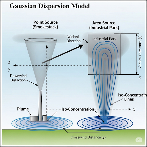
Gaussian Dispersion Model
🔒 Unlock Audio Lesson
Sign up and enroll to listen to this audio lesson

Let's focus specifically on the Gaussian dispersion model now. What do you think makes this model popular?
It's probably because it provides quick estimates of pollutant concentrations.
Exactly! It's often used as a screening tool. Can anyone summarize what the basic equation looks like?
It accounts for emission rate, wind speed, and dispersion parameters like sigma y and sigma z.
Perfect! Remember: 'Q for concentration, U for wind speed'. Now, what happens when we have multiple sources?
We might think it increases concentrations, but it doesn’t always add linearly.
Absolutely correct! We see that interactions can lead to decreased cumulative impact. That’s a key point to remember!
Comparative Modeling Frameworks
🔒 Unlock Audio Lesson
Sign up and enroll to listen to this audio lesson
Now let's differentiate between AERMOD and CALPUFF. Who can describe AERMOD?
AERMOD is a steady-state model that requires meteorological data.
Correct! In contrast, what does CALPUFF offer?
CALPUFF can model both steady-state and non-steady-state situations, like explosions.
Exactly! CALPUFF’s versatility is key in certain scenarios. What's essential in both models?
We need to input the source characteristics like emission rates and stack information.
Very good! Remember: 'Data drives models!' A final recap: AERMOD is simple and steady-state, while CALPUFF is versatile!
Introduction & Overview
Read summaries of the section's main ideas at different levels of detail.
Quick Overview
Standard
The section elaborates on dispersion models, specifically Gaussian dispersion models, and their implementation for understanding air quality in different geographical contexts. It highlights how these models can vary based on the characteristics of the emissions, sources, and local environmental factors.
Detailed
Environmental Quality: Monitoring and Analysis
This section delves into the essential concepts of dispersion models used in environmental quality monitoring, emphasizing the Gaussian dispersion model. The discussion begins with a recap of point and area sources, describing how dispersion can be evaluated relative to different origins and how adjustments must be made based on multiple contributing factors, including local circulation effects. The section further explores the complexities around additive contributions from multiple sources, noting experimental evidence suggesting that the sum of individual contributions does not equate to simple addition due to interaction effects. Furthermore, different modeling frameworks such as AERMOD and CALPUFF are introduced, highlighting their data requirements and operational mechanics. A detailed look at the regulatory context in which these models operate provides insights into their practical applications. Understanding these models is critical for effective environmental quality assessment and compliance with regulatory standards.
Youtube Videos


Audio Book
Dive deep into the subject with an immersive audiobook experience.
Introduction to Line Sources
Chapter 1 of 5
🔒 Unlock Audio Chapter
Sign up and enroll to access the full audio experience
Chapter Content
There are some line sources. So in the line source equation, this q is different. You can see that the equation is slightly different because σ, is considered negligible. This is a continuous road extending infinitely and your wind is coming perpendicularly here, so it is a crosswind.
Detailed Explanation
Line sources refer to continuous emissions spread over an extended area, like a busy road from which vehicles emit pollutants. In analysis, the term 'q' (the emission rate) is distinct because it applies to this continuous source. When emissions come from a line source, the dispersion calculations consider the road as infinitely long, allowing simplifications in the mathematical models.
Examples & Analogies
Think of a line source like a train running on a railway track. As the train moves, it emits smoke and gases continuously along the track. Here, we view the train track as a long line where emissions occur at many points, rather than a single point, simplifying how we analyze pollution spread.
Emissions Along the Line
Chapter 2 of 5
🔒 Unlock Audio Chapter
Sign up and enroll to access the full audio experience
Chapter Content
Emission is occurring this direction, all the vehicles are traveling on this road. So you will have one plume like this, the next plume like this, next plume like this, next plume like this, that is what crosswind compensation is equivalent to having the same thing.
Detailed Explanation
As vehicles travel along the road, they emit pollutants that form plumes. In a crosswind condition, these plumes can drift away from their source, affecting air quality in surrounding areas. The idea of 'crosswind compensation' helps in understanding how the wind influences the dispersion of these plumes, allowing us to predict where the pollutants will go and their concentrations in areas downwind.
Examples & Analogies
Imagine you're blowing smoke from a birthday candle. If there’s a fan blowing air across the room, the smoke won't just rise straight up; it will drift sideways with the wind. Similarly, vehicles on a busy road emit pollutants that can be pushed away by crosswinds, spreading the pollution over a larger area.
Understanding Line Source Equations
Chapter 3 of 5
🔒 Unlock Audio Chapter
Sign up and enroll to access the full audio experience
Chapter Content
So, for a given section of the road, you can calculate using this. Then of course q you have to calculate by doing you need to know what are the vehicles on the road and the emission factor based on composition of vehicles.
Detailed Explanation
In order to calculate the pollutant concentration from a line source, we need to know the emission rate 'q.' This is determined by counting the number of vehicles and understanding their emissions based on vehicle types (such as cars vs. trucks). Each type of vehicle has a different amount of pollutants it releases, thus requiring accurate data collection for effective modeling.
Examples & Analogies
Think of it like baking cookies. If you want to know how sweet the cookies will be, you must know not only how many cookies you're baking but also how much sugar each cookie recipe calls for. Similarly, we must gather data on vehicle types and their respective emissions to accurately model the pollution they produce.
Factoring Vehicle Dynamics
Chapter 4 of 5
🔒 Unlock Audio Chapter
Sign up and enroll to access the full audio experience
Chapter Content
Collection of that data is fairly laborious to do and you have to keep doing it again and again because these things will change with time, because in the morning time vehicles will travel fast and peak time vehicles will travel slowly and so on.
Detailed Explanation
Data on vehicle numbers and behavior is not static. Traffic patterns fluctuate throughout the day, with variations in vehicle speed and count depending on rush hours. Collecting and analyzing this data helps create a more accurate depiction of emissions over time, but it requires ongoing effort and adjustment as conditions change.
Examples & Analogies
Imagine you are trying to estimate the number of people visiting a park daily. On weekends, more people come, and their visiting hours vary. If you only observe for a day, you won't have the full picture. You would need to study various times across different days for a more accurate estimate. Similarly, we must continuously monitor traffic and emissions to understand their impact holistically.
Impact of Wind Direction on Calculations
Chapter 5 of 5
🔒 Unlock Audio Chapter
Sign up and enroll to access the full audio experience
Chapter Content
This is an extension of this again when you have an angle. The wind speed is not at right angles, it is an angle to the road, this can happen. So there is another term here called sin(φ) here.
Detailed Explanation
Wind direction plays a crucial role in dispersing emissions from a line source. When wind approaches at an angle rather than straight across the road, we have to adjust calculations using the sine of the angle (φ). This adjustment allows for a more accurate understanding of how pollutants will spread in the environment, ensuring better air quality predictions.
Examples & Analogies
Imagine standing on the beach, where the wind usually comes straight in from the ocean. If you start walking at an angle toward the water, the wind will now hit you at an angle, and the sand will scatter differently compared to a direct onslaught. The same principle applies to how wind affects the direction pollutants spread from a line source—angle matters!
Key Concepts
-
Point Source: A specific source of emissions identified at a particular location.
-
Gaussian Dispersion Model: An efficient modeling approach for estimating pollutant dispersal assuming a normal distribution.
-
AERMOD: A regulatory modeling tool considered suitable for steady-state conditions.
-
CALPUFF: A versatile model that can handle varying conditions in air quality monitoring.
Examples & Applications
Modeling the emissions from a factory as a point source to assess air quality in surrounding neighborhoods using AERMOD.
Using CALPUFF to analyze the dispersion of pollutants from a highway during peak traffic hours.
Memory Aids
Interactive tools to help you remember key concepts
Rhymes
If pollutants spread like a wave, Gaussian's the model that we save.
Stories
Imagine a factory emitting smoke. If we treat that point like a drop in water, how do the ripples spread? That’s the Gaussian approach.
Memory Tools
When modeling dispersion, remember 'A for AERMOD, C for CALPUFF'—these help you identify suitable models!
Acronyms
P for Point, A for Area—sources we must consider with care-a!
Flash Cards
Glossary
- Dispersion Model
A mathematical framework to predict the spread of pollutants in the environment.
- Gaussian Model
A type of dispersion model that assumes a normal distribution of pollutant concentrations.
- AERMOD
A regulatory model used for steady-state dispersion modeling by the American Meteorological Society.
- CALPUFF
A modeling system for simulating the dispersion of air pollutants, allowing for non-steady-state applications.
- Point Source
A single, identifiable source of pollution that can be characterized spatially.
Reference links
Supplementary resources to enhance your learning experience.