5 - Plume Dynamics

Today, we're discussing dispersion models used in environmental engineering. These models help us predict how pollutants spread in the atmosphere from various sources. Can anyone tell me what they think a dispersion model is?

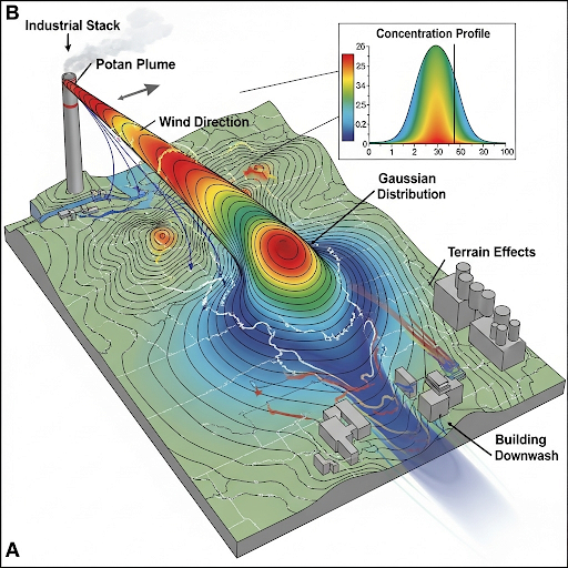
Exactly! It predicts the concentration and distribution of a pollutant based on its source, like a chimneys' emissions. We typically start with the Gaussian dispersion model. The term 'Gaussian' refers to the bell-shaped distribution of pollutants in the air.

Not quite. The model simplifies that aspect but in reality, pollutants can be affected by wind and other factors. Remember this: 'Gaussian' is about predicting trends, but we must adjust for actual conditions. Can anyone think of factors that might necessitate these adjustments?

Right! Also, geographic factors. We'll dive into that next.

**Summary**: Today, we learned that dispersion models predict pollutant spread based on the source and environmental conditions, notably starting with the Gaussian model.

Let's expand on dispersion sources. What’s the difference between a point source and an area source?

Exactly! If we model an area source, we consider uniform emissions across a broader region. It's crucial to adjust our models based on how zoomed in or out we are. Can you visualize how this would affect our calculations?

Exactly! This oversimplifies the reality. Thus, proper modeling ensures accurate predictions. Keep in mind, how would you use data differently if modeling for a city versus a small neighborhood?

Yes! And remember to consider local meteorological data for such analyses. That’s an essential factor in dispersion modeling.

**Summary**: We learned that point and area sources require different modeling approaches, particularly regarding the scale of emissions and the necessity for localized data.

Today, let’s talk about the effects when we have multiple pollutant sources. Can anyone guess how their contributions would work?

Great question! It’s actually more complex. Experimental evidence shows that sometimes the contributions are less than simply additive. We describe this relationship with a factor, often less than one. Let’s think: why might that occur?

Spot on! Turbulence and dispersion dynamics can significantly affect outcomes. So, don’t simply assume additions of pollutants will equal expected concentrations. Real-world complexities must be factored in.

**Summary**: We discussed how multiple sources could interact non-linearly in their contributions to pollution dispersion, highlighting the need to consider dynamics like turbulence.

Let’s shift now to Regulatory Models. Have any of you heard about AERMOD or CALPUFF?

Correct! AERMOD is the regulatory model primarily for steady-state emissions. In contrast, CALPUFF uses a puff model, accounting for non-steady emissions. What do you think are key elements we need to input into these models?

Exactly! We also require source data—emission rates, stack heights, and even meteorological conditions. Remember that if you lack some of that data, you might prefer using ISC instead.

Great point! Models are validated against real-world data through field experiments where pollutants are released and monitored. This helps ensure reliability.

**Summary**: In reviewing regulatory models like AERMOD and CALPUFF, we noted the importance of specific input data and the critical role of validating these models with real-world experiments.

Finally, let's discuss how we prove that our dispersion models work. How do we validate a model?

Precisely! Field experiments often involve releasing tracers to see how they disperse under real conditions. What’s a challenge we might face during these validations?

Exactly! Conditions like wind patterns and temperature fluctuations affect dispersion, making it tricky to capture precise data. It's crucial to also consider how different terrains might influence plume behavior as well.

**Summary**: We discussed the critical role of validation in dispersion modeling using field experiments and how various environmental factors must be accounted for in this process.