Today, we are diving into the crucial topic of numerical methods for simulating complex root behavior in differential equations. Why do you think we need numerical methods, Student_1?

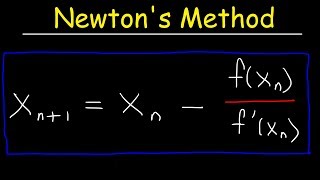
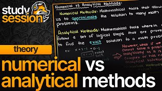
Exactly! Analytical solutions can be challenging or even impossible for certain equations. Numerical methods, such as Runge-Kutta and Euler’s Method, help us approximate these solutions instead.

The Runge-Kutta method is a powerful technique for numerical approximation of solutions to ODEs. It systematically improves accuracy through multiple estimations. Remember, 'Runge-Runs Right' — it's about getting accurate estimates!

Certainly! Numerical methods allow engineers to simulate and predict the system's behavior, especially when faced with complex roots, ensuring structures can withstand dynamic loads. They are vital for safety and design optimization.

Yes, both MATLAB and Python offer comprehensive capabilities for implementing these numerical techniques. Remember, effective structuring in code can lead to accurate simulations. 'Good structure, good simulation!'

Numerical simulations allow real-time health monitoring, ensuring If complex root behavior is detected, engineers can respond promptly. This is crucial for maintaining structural integrity.

Now, let's delve deeper into the process of converting second-order differential equations into a system of first-order ODEs. Who can explain why this conversion is necessary?

Exactly! By breaking it down into first-order equations, we handle each equation more simply. Also, remember: 'First is best for solving!'— this highlights the benefit of breaking down complexities.

Certainly! For the differential equation \(\frac{d^2y}{dt^2} + 6\frac{dy}{dt} + 25y = 0\), we translate it to a system where \(y_1 = y\) and \(y_2 = \frac{dy}{dt}\). This gives us two first-order equations: \(\frac{dy_1}{dt} = y_2\) and \(\frac{dy_2}{dt} = -6y_2 - 25y_1\).

Absolutely! Once formulated, these first-order equations can be tackled using methods like Runge-Kutta or Euler’s approach, allowing us to effectively simulate the system's behavior.

Choosing the right step size and method is crucial for accuracy. Remember, ‘Small steps equal big precision!’ By optimizing these, we achieve reliable simulations.

To wrap up, let’s reflect on what we've learned about numerical methods and their applications in civil engineering. What stood out to you, Student_2?

Indeed, they provide engineers with critical insights. Remember, understanding these simulations enhances structural safety. Anyone else want to share?

Precisely, and let's not forget the tools available, such as MATLAB and Python, which can effectively implement these methods. 'Tools are keys to success!'

That’s a great takeaway! In summary, understanding numerical methods equips future engineers like yourselves with the essential skills to optimize safety and performance in civil structures.