
Derivation of the Variation of Parameters Formula
Enroll to start learning
You’ve not yet enrolled in this course. Please enroll for free to listen to audio lessons, classroom podcasts and take practice test.
Interactive Audio Lesson
Listen to a student-teacher conversation explaining the topic in a relatable way.
Introducing Variation of Parameters
🔒 Unlock Audio Lesson
Sign up and enroll to listen to this audio lesson

Today, we're diving into the derivation of the variation of parameters formula. Can anyone tell me what a non-homogeneous differential equation is?

It's an equation that includes a non-homogeneous term, right? Like an external force or input?
Exactly! This section deals with equations of the form `y'' + p(x)y' + q(x)y = g(x)`, where `g(x)` is that non-homogeneous term. Now, how do you think these equations are solved?

By finding the general solution for the homogeneous part and then adding a particular solution?
Precise! The variation of parameters helps us find that particular solution. Remember, it's powerful because it can handle a variety of forcing functions!

So, we start with a known solution to the homogeneous equation?
Correct! We utilize two linearly independent solutions of the homogeneous equation to construct our particular solution.

How do we differentiate that assumption?
Great question! We differentiate our assumed solution while applying some constraints, which helps simplify our equations. Let's move to that derivation next.
Differentiating and Applying Constraints
🔒 Unlock Audio Lesson
Sign up and enroll to listen to this audio lesson

Now, when we differentiate our assumed solution `y_p(x) = u_1(x)y_1(x) + u_2(x)y_2(x)`, what do we impose for simplification?
We impose the constraint `u_1'(x)y_1(x) + u_2'(x)y_2(x) = 0`.
Exactly! This constraint allows us to eliminate some terms when differentiating again. Can someone help me with the benefit of this step?
It simplifies the math significantly, so we can focus on solving the system of equations that arises.
Well put! After substituting into our original differential equation, we obtain two equations we can solve using Cramer’s rule.
And the Wronskian `W(x)` is crucial here, right?
Absolutely. The Wronskian determines the behavior of the solutions. Let's take this to the next step.
Solving for Coefficients
🔒 Unlock Audio Lesson
Sign up and enroll to listen to this audio lesson
As we derive `u_1(x)` and `u_2(x)` using the Wronskian, can anyone remind me how we express these coefficients?
We’ve got `u_1(x) = - rac{y_2(x)g(x)}{W(x)}` and `u_2(x) = rac{y_1(x)g(x)}{W(x)}`.
Excellent! Now that we have them, what's the next step in our process?
We integrate `u_1(x)` and `u_2(x)` to get the functions needed for our particular solution.
Exactly correct! Once we have those integrated, we can construct the particular solution. What does it look like?
`y_p(x) = u_1(x)y_1(x) + u_2(x)y_2(x)`.
Right! And then we add it to the general solution of the homogeneous equation. Great work today, everyone!
Introduction & Overview
Read summaries of the section's main ideas at different levels of detail.
Quick Overview
Standard
This section explains how to derive the variation of parameters formula used in the context of non-homogeneous second-order linear differential equations. It involves differentiating a particular solution that is expressed in terms of linearly independent solutions of the corresponding homogeneous equation and applying constraints to simplify calculations.
Detailed
Derivation of the Variation of Parameters Formula
In this section, we explore the derivation of the variation of parameters formula, fundamental in finding particular solutions to non-homogeneous second-order linear differential equations, where the typical method of undetermined coefficients may not apply. The process begins with recognizing that a particular solution can be represented as a linear combination of two known solutions to the homogeneous equation. By differentiating this proposed solution while applying a specific constraint to simplify terms, we subsequently derive a system of linear equations involving functions that are easily solvable using determinants. This approach notably employs the Wronskian of the independent solutions, which plays a crucial role in determining the coefficients of the particular solution. The validity and application of this method extend to various engineering contexts, showcasing its utility in real-world problem-solving.
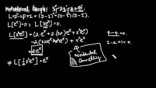
Youtube Videos


Audio Book
Dive deep into the subject with an immersive audiobook experience.
Differentiating the Assumed Particular Solution
Chapter 1 of 9
🔒 Unlock Audio Chapter
Sign up and enroll to access the full audio experience
Chapter Content
Differentiate y (x):
p
y (x)=u (x)y (x)+u (x)y (x)+u (x)y (x)+u (x)y (x)
p′ 1′ 1 1′ 2′ 2 2 2′
Detailed Explanation
In this step, we begin to find the particular solution for the non-homogeneous differential equation. We differentiate the assumed form of our particular solution, which is expressed in terms of two functions, u₁(x) and u₂(x), multiplied by the homogeneous solutions y₁(x) and y₂(x). This differentiation allows us to manipulate the equation further to ultimately solve for the unknown functions u₁ and u₂. It highlights that we are dealing with two dynamic parts that will contribute to the change in our dependent variable y.
Examples & Analogies
Think of differentiating the assumed solution as taking a snapshot of an ongoing process. Just like observing how much a car has traveled over time can be described by measuring its speed at different moments, here, we're observing how changes in the functions u₁ and u₂ affect the overall behavior of the solution y.
Imposing a Constraint
Chapter 2 of 9
🔒 Unlock Audio Chapter
Sign up and enroll to access the full audio experience
Chapter Content
To simplify the derivation, we impose a constraint:
u (x)y (x)+u (x)y (x)=0
1′ 1 2′ 2
Detailed Explanation
To make our equations manageable, we impose a constraint between the derivatives of the functions u₁ and u₂ and the homogeneous solutions y₁ and y₂. This constraint reduces the complexity of our differentiation results and is pivotal in applying the variation of parameters method. It ensures that the changes we analyze in our solution do not contribute to interference when we substitute back into the original equation.
Examples & Analogies
Imagine you are tuning an instrument. By adjusting a certain string while keeping another string still, you're optimizing the sound without creating discord. The constraint we apply functions similarly by ensuring that while we modify u₁ and u₂, they must work harmoniously together with y₁ and y₂.
Second Differentiation
Chapter 3 of 9
🔒 Unlock Audio Chapter
Sign up and enroll to access the full audio experience
Chapter Content
Differentiate again:
y (x)=u (x)y (x)+u (x)y (x)+u (x)y (x)+u (x)y (x)
p′′ 1′ 1′ 1 1′′ 2′ 2′ 2 2′′
Detailed Explanation
In this step, we differentiate the partially derived form of y again to obtain a second derivative. This robust differentiation is crucial as it captures more detailed behavior of our assumed particular solution and facilitates substitution into the non-homogeneous equation. At this point, we are preparing to fully integrate the results into the main equation to derive our solution for u₁ and u₂.
Examples & Analogies
Consider measuring the height of a person as they grow. The first differentiation tells us the speed of growth (how fast they are growing), while the second differentiation tells us if that growth speed is increasing or tapering off. This deeper insight helps us predict future heights more accurately, just as our second derivative will aid in finding precise functions for our solution.
Substitution into the Original Equation
Chapter 4 of 9
🔒 Unlock Audio Chapter
Sign up and enroll to access the full audio experience
Chapter Content
Now substitute y ,y ,y into the original non-homogeneous equation:
p p′ p′′
y +p(x)y +q(x)y =g(x)
Detailed Explanation
Now that we have our differentiated forms ready, we substitute them into the original non-homogeneous differential equation. This is where we apply all our work into one cohesive form. With this substitution, we will reveal relationships that directly lead us to forming a system of equations for u₁ and u₂. It allows us to directly link the coefficients of the non-homogeneous terms to our modified solutions.
Examples & Analogies
Think of this step as putting together a puzzle where you've spent significant time on the edges and corners. Now, as you substitute everything into the full picture, you begin to see the connections and relationships between the pieces, ultimately leading you to the completed image.
Setting Up the System of Equations
Chapter 5 of 9
🔒 Unlock Audio Chapter
Sign up and enroll to access the full audio experience
Chapter Content
After substituting and simplifying using the homogeneous equation, we get:
u (x)y (x)+u (x)y (x)=g(x)
1′ 1′ 2′ 2′
Detailed Explanation
After performing the necessary substitutions and simplifications, we arrive at a system of two linear equations that involve our unknown functions u₁(x) and u₂(x). This step condenses our calculations into a manageable format that allows us to use algebraic methods (like Cramer's rule) or matrix techniques for solving systems. These equations express how the particular solution is directly influenced by different factors in the non-homogeneous term g(x).
Examples & Analogies
This process is similar to solving for variables in a budget. When you have multiple expenses (like rent, food, and entertainment) that must add up to a total budget, you can set up equations based on your knowns and unknowns to find out how much you can spend on each category.
Using the Wronskian for Coefficients
Chapter 6 of 9
🔒 Unlock Audio Chapter
Sign up and enroll to access the full audio experience
Chapter Content
Let W(x) be the Wronskian of y and y :
W(x)=y (x)y (x)−y (x)y (x)
1 2′ 1′ 2
Detailed Explanation
We define W(x) as the Wronskian, which is a determinant used to determine whether our two homogeneous solutions y₁ and y₂ are independent solutions. The Wronskian plays a crucial role in finding the coefficients u₁ and u₂. If W(x) is zero, the functions are not independent, meaning we cannot use them effectively in the variation of parameters method. This determinant is essential for ensuring our solution's viability and correctness.
Examples & Analogies
Think of the Wronskian as a test of collaboration between two team members on a project. If they have distinct skills (independent solutions), they complement each other well. However, if both have the same skills (dependent solutions), their collaboration isn't as effective. The Wronskian tests this collaboration.
Finding the Coefficients u₁ and u₂
Chapter 7 of 9
🔒 Unlock Audio Chapter
Sign up and enroll to access the full audio experience
Chapter Content
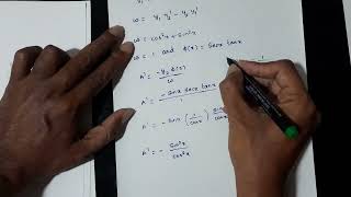
Then:
u (x)=−
y (x)g(x) , u (x)=
y (x)g(x)
1′ W(x) 2′ W(x)
Detailed Explanation
Based on our earlier system, we derive equations for u₁ and u₂ using the Wronskian. The formulas express how the particular solutions are weighted by the impact of the forcing function g(x) and the relationships captured in the Wronskian. By deriving u₁ and u₂ through these relations, we are systematically allocating the influence of g(x) across our homogeneous solutions.
Examples & Analogies
Imagine you have a recipe that requires a certain proportion of different spices (influences from y solutions) to achieve a desired taste (the outcome from g). Each spice contributes differently, analogous to how u₁ and u₂ bring the right balance to solve for the particular solution.
Integrating to Find u₁ and u₂
Chapter 8 of 9
🔒 Unlock Audio Chapter
Sign up and enroll to access the full audio experience
Chapter Content
Now integrate both:
Z y (x)g(x) Z y (x)g(x)
u (x)=− 2 dx, u (x)= 1 dx
1 W(x) 2 W(x)
Detailed Explanation
To finalize our solution, we need to integrate the expressions derived for u₁ and u₂. These integrals provide us with the specific forms of our functional coefficients that we can utilize in the formulation of our particular solution. This step essentially transforms our relationships into solvable functions that play a critical role in determining the overall solution to the differential equation.
Examples & Analogies
When you mix ingredients, like when you bake, there's a moment where just mixing them is not enough – you have to 'cook' it (integrate) to achieve the final dish. Here, ‘cooking’ through integration turns our raw functional relationships into usable forms.
Constructing the Particular Solution
Chapter 9 of 9
🔒 Unlock Audio Chapter
Sign up and enroll to access the full audio experience
Chapter Content
Thus, the particular solution is:
Z y (x)g(x) Z y (x)g(x)
y (x)=−y (x) 2 dx+y (x) 1 dx
p 1 W(x) 2 W(x)
Detailed Explanation
After integrating, we construct the final form of the particular solution by combining u₁ and u₂ with the homogeneous solutions y₁ and y₂. This final formula is hugely significant as it gives us the particular solution to the non-homogeneous equation we started with. It marks the culmination of our systematic process and provides insight into how the solution encompasses both the natural behavior (homogeneous solution) and the imposed external effects (particular solution).
Examples & Analogies
Think of this as putting on the final touches to a painting. You have the base colors (homogeneous solutions) and you mix in highlights and shadows (particular solutions) to create a complete and vibrant artwork. This step signifies bringing together all elements into a definitive form.
Key Concepts
-
The variation of parameters method solves non-homogeneous differential equations using known solutions of the homogeneous counterpart.
-
The Wronskian is essential for determining the behavior and independence of solutions to differential equations.
Examples & Applications
For the differential equation y'' + p(x)y' + q(x)y = g(x), we find the particular solution using known solutions of the homogeneous form; example cases include exponential, trigonometric inputs.
In engineering practice, calculating beam deflection subjected to arbitrary forces can employ variation of parameters for determining a particular solution efficiently.
Memory Aids
Interactive tools to help you remember key concepts
Rhymes
To find where solutions play, use Wronskian’s sway, independence on display!
Stories
Imagine a hawk and a dove soaring together in a breeze. The hawk orients based on freedom while the dove remains tethered, just like the independence of our solutions defined by the Wronskian.
Memory Tools
Remember: SUDS – Solve, Use, Differentiate, Solve for coefficients.
Acronyms
VIP - Variation, Independent Solutions, Particular solutions.
Flash Cards
Glossary
- NonHomogeneous Differential Equation
A differential equation that includes a non-zero term that does not depend on the dependent variable.
- Variation of Parameters
A method to find particular solutions to non-homogeneous differential equations using the known solutions of the corresponding homogeneous equation.
- Wronskian
A determinant associated with a set of solutions to a differential equation, used to determine their linear independence.
- Determinants
A mathematical object that can be computed from the elements of a square matrix and encodes certain properties about the matrix.
Reference links
Supplementary resources to enhance your learning experience.