General Form of a Non-Homogeneous Second-Order Linear Differential Equation
Enroll to start learning
You’ve not yet enrolled in this course. Please enroll for free to listen to audio lessons, classroom podcasts and take practice test.
Interactive Audio Lesson
Listen to a student-teacher conversation explaining the topic in a relatable way.
General Form of the Equation
🔒 Unlock Audio Lesson
Sign up and enroll to listen to this audio lesson

Today we'll explore the general form of a non-homogeneous second-order linear differential equation. Can anyone tell me the equation's structure?

It’s in the form y′′ + p(x)y′ + q(x)y = g(x).

Correct! Now, what do each of these components represent?

y is the dependent variable, like displacement, right?

Yes, exactly! And what's the role of g(x)?

That's the non-homogeneous term – the external force acting on the system.

Great job! Now, let’s summarize: we’re dealing with a model where y represents a system's response influenced by external factors.
Components of the Equation
🔒 Unlock Audio Lesson
Sign up and enroll to listen to this audio lesson

Let’s break down the terms further. What are p(x) and q(x)?

They are coefficient functions that describe the system's behavior.

Exactly! What happens to our equation if p(x) or q(x) changes?

It would change the dynamics of the system we are modeling.

Right! That's why understanding these components is crucial for proper modeling.
General and Particular Solutions
🔒 Unlock Audio Lesson
Sign up and enroll to listen to this audio lesson

Now, let’s discuss the solutions to the differential equation. What are the two types of solutions?

The general solution y_h and the particular solution y_p.

Correct! How do these solutions work together?

They combine to form the complete solution of the equation: y(x) = y_h(x) + y_p(x).

So, y_h handles the inherent behavior while y_p deals with external influences?

Absolutely! This combination allows us to fully describe the system's behavior.
Introduction & Overview
Read summaries of the section's main ideas at different levels of detail.
Quick Overview
Standard
In this section, we detail the structure of the non-homogeneous second-order linear differential equation, represented as y′′+p(x)y′+q(x)y = g(x). We discuss the function components and the general solution, explaining how this framework is applicable in various engineering contexts.
Detailed
General Form of a Non-Homogeneous Second-Order Linear Differential Equation
This section presents the standard form of a second-order linear non-homogeneous differential equation, which is essential in solving complex engineering problems. The equation is expressed as:
$$y^{\prime\prime} + p(x)y^{\prime} + q(x)y = g(x)$$
Where:
- y is the dependent variable, representing measurements like displacement or temperature.
- x is the independent variable, such as time or distance.
- p(x) and q(x) are coefficient functions which define the system's behavior.
- g(x) is the non-homogeneous term, an external influence affecting the system.
The solution comprises two parts:
1. Homogeneous Solution $y_h(x)$: The general solution to the associated homogeneous equation.
2. Particular Solution $y_p(x)$: A specific solution that accounts for the non-homogeneous term g(x).
Thus, the overall solution is expressed as:
$$y(x) = y_h(x) + y_p(x)$$
The flexibility of this model allows it to accommodate various external influences, making it applicable across diverse engineering applications.
Youtube Videos
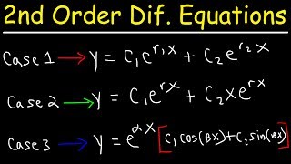


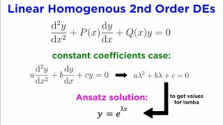
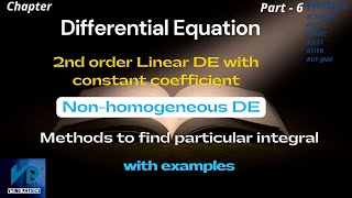
Audio Book
Dive deep into the subject with an immersive audiobook experience.
General Form of the Equation
Chapter 1 of 3
🔒 Unlock Audio Chapter
Sign up and enroll to access the full audio experience
Chapter Content
A general second-order linear non-homogeneous differential equation is given by:
y′′ + p(x)y′ + q(x)y = g(x)
Detailed Explanation
This equation represents a relationship where the dependent variable y has its second derivative y′′, its first derivative y′, and the function y itself influenced by variable coefficients p(x) and q(x). The right-hand side, g(x), represents external forces or inputs affecting the system, making the equation non-homogeneous.
Examples & Analogies
Think of this equation as a simple model of a swing. Here, y represents the position of the swing, p(x) and q(x) could represent friction and swing length, respectively, while g(x) represents the push you give it (like a push from a friend). Just as the swing's movement is influenced by these factors, the solution to this equation gives us insights into how the system behaves under various influences.
Variables and Functions Defined
Chapter 2 of 3
🔒 Unlock Audio Chapter
Sign up and enroll to access the full audio experience
Chapter Content
Where:
yis the dependent variable (typically displacement, temperature, etc.)xis the independent variable (time, distance, etc.)p(x), q(x): Coefficient functionsg(x): Non-homogeneous term (external input or forcing function)
Detailed Explanation
In this equation, y can be thought of as the outcome we want to understand—like the displacement of a beam under pressure. The independent variable x tells us how the situation changes; for instance, as time progresses or as we move along a beam. The functions p(x) and q(x) add complexity, representing how factors like material properties change with position or time. Finally, g(x) captures any external effects, like wind on a bridge or changes in temperature.
Examples & Analogies
Imagine you're baking a cake. The position of the cake (how it rises and sets) is like the dependent variable y. The time you're baking it (which gradually changes) is your independent variable x. The oven temperature (which might not be constant) can represent p(x) and q(x), while any additional ingredients (like frosting added afterward) influence the final product, represented by g(x). Each element plays its part in affecting the outcome of the cake!
Solution of the Differential Equation
Chapter 3 of 3
🔒 Unlock Audio Chapter
Sign up and enroll to access the full audio experience
Chapter Content
The solution to this equation is given by:
y(x) = y_h(x) + y_p(x)
Where:
y_h(x): General solution to the homogeneous equationy′′ + p(x)y′ + q(x)y = 0y_p(x): Particular solution to the non-homogeneous equation.
Detailed Explanation
The total solution to our differential equation combines two parts: the homogeneous solution y_h(x) and the particular solution y_p(x). The homogeneous solution represents the system's natural behavior without any external inputs, while the particular solution addresses the effects of those external inputs or adjustments. Together, they provide a complete picture of how the system behaves under both natural and forced conditions.
Examples & Analogies
Continuing with our swing analogy, y_h(x) is akin to how the swing moves on its own when you let it go, capturing the natural swing dynamics. y_p(x), however, represents how far the swing moves when someone pushes it. The total movement (y(x)) of the swing at any moment is the combination of its natural motion plus the added push from your friend!
Key Concepts
-
General Form: y′′ + p(x)y′ + q(x)y = g(x) represents the model.
-
Homogeneous Solution: Represents the natural response of the system.
-
Particular Solution: Represents the response due to external influences.
Examples & Applications
An example of a second-order linear non-homogeneous equation is y′′ + 2y′ + 3y = sin(x).
This equation could model oscillations in a mechanical system under a forcing function represented by sin(x).
Memory Aids
Interactive tools to help you remember key concepts
Rhymes
In equations where y can sway, p and q show the way. g’s the force that comes to play, guiding y both night and day.
Stories
Imagine a boat (y) on a river (x), the currents (g) change with seasons affecting how the boat travels. The banks (p and q) guide the boat's journey.
Memory Tools
To remember the equation's form: 'y' is where we aim, 'p' helps frame, 'q' leads the game, 'g' is the claim!
Acronyms
For y = g
= Grounded – representing total response involving both homogenous and heterogeneous parts.
Flash Cards
Glossary
- NonHomogeneous
Refers to differential equations with an external forcing function or input, represented by g(x).
- Dependent Variable
The variable that depends on another variable, typically associated with output measures in the differential equation.
- Independent Variable
The variable that can be controlled or is input, typically time or distance.
- Coefficient Function
Functions p(x) and q(x) that influence the behavior of the dependent variable in the equation.
Reference links
Supplementary resources to enhance your learning experience.
