
Principle of the Variation of Parameters
Enroll to start learning
You’ve not yet enrolled in this course. Please enroll for free to listen to audio lessons, classroom podcasts and take practice test.
Interactive Audio Lesson
Listen to a student-teacher conversation explaining the topic in a relatable way.
Introduction to Variation of Parameters
🔒 Unlock Audio Lesson
Sign up and enroll to listen to this audio lesson

Today, we're diving into the Principle of Variation of Parameters, a method for solving non-homogeneous linear differential equations. So, can anyone tell me what a non-homogeneous equation looks like?

Is it something like y'' + p(x)y' + q(x)y = g(x)?
Exactly! And we know how to solve the homogeneous part, right? What does the general solution to a homogeneous equation look like?

It’s C1y1 + C2y2, where y1 and y2 are the independent solutions.
Perfect! Now, to find a particular solution, we assume it's in the form of u1y1 + u2y2. Let's remember this as 'two u's make the particular'.

Got it! The two u's are for the particular solution!
Finding u1 and u2
🔒 Unlock Audio Lesson
Sign up and enroll to listen to this audio lesson

Now, in order to find u1 and u2, we differentiate our expression for y_p and apply a constraint that simplifies our work. Can anyone recall what this constraint is?

Is it u1'y1 + u2'y2 = 0?
Exactly! This constraint helps us reduce the complexity. After we differentiate and substitute into the original equation, we get a system to solve for u1 and u2.
And we can use Cramer’s rule to solve this system, right?
Absolutely! Cramer’s rule is a powerful tool for finding u1 and u2. Let's repeat: apply the constraint, differentiate, substitute, and solve the system.
Constructing the Complete Solution
🔒 Unlock Audio Lesson
Sign up and enroll to listen to this audio lesson
Once we have the particular solution, how do we construct the complete solution to our differential equation?
We combine the homogeneous solution and the particular solution!
Correct! The overall solution will be y(x) = y_h(x) + y_p(x). Now, why is the Variation of Parameters preferred in many engineering applications?
It’s more versatile! It accommodates different forms of g(x) that undetermined coefficients cannot handle.
Well stated! And let’s keep in mind that the integration required in this process can be computationally intensive.
Introduction & Overview
Read summaries of the section's main ideas at different levels of detail.
Quick Overview
Standard
This section describes the Principle of Variation of Parameters, highlighting its ability to derive particular solutions for non-homogeneous linear differential equations. It builds upon previous knowledge of the homogeneous equation and introduces a systematic approach to finding solutions that accommodate a wider range of non-homogeneous terms compared to the method of undetermined coefficients.
Detailed
Detailed Summary
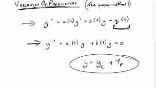
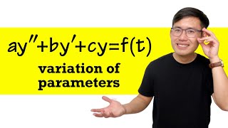
The Principle of Variation of Parameters is a powerful technique used to find particular solutions to non-homogeneous linear differential equations of the form:
$$ y'' + p(x)y' + q(x)y = g(x) $$
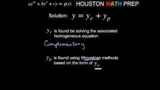
This method assumes that the solutions to the corresponding homogeneous equation, $$ y'' + p(x)y' + q(x)y = 0 $$, are known. Let these solutions be $$ y_1(x) $$ and $$ y_2(x) $$, forming the general solution:
$$ y_h(x) = C_1 y_1(x) + C_2 y_2(x) $$
For the non-homogeneous part, we posit a particular solution of the form:
$$ y_p(x) = u_1(x) y_1(x) + u_2(x) y_2(x) $$
where $$ u_1(x) $$ and $$ u_2(x) $$ are functions yet to be determined. By differentiating $$ y_p(x) $$ and imposing a constraint that simplifies the derivatives (specifically $$ u_1' y_1 + u_2' y_2 = 0 $$), you can derive a system of equations to solve for $$ u_1 $$ and $$ u_2 $$ using Cramer’s rule.
The resulting particular solution, when combined with the homogeneous solution, yields the complete solution to the differential equation. The method is especially versatile as it can handle a broader range of forcing functions compared to the undetermined coefficients method. Engineering applications, such as beam deflection and vibration analysis, benefit greatly from this method.
Youtube Videos


Audio Book
Dive deep into the subject with an immersive audiobook experience.
Homogeneous Equation and General Solution
Chapter 1 of 2
🔒 Unlock Audio Chapter
Sign up and enroll to access the full audio experience
Chapter Content
Suppose we already have the solution to the corresponding homogeneous equation:
y′′+p(x)y′+q(x)y =0
Let the two linearly independent solutions of the homogeneous part be y₁(x) and y₂(x). Then the general solution of the homogeneous equation is:
yh(x)=C₁y₁(x)+C₂y₂(x)
Detailed Explanation
The section begins by assuming we have already solved the homogeneous equation, which does not include the forcing function (the right side of the equation). The homogeneous equation is represented as y′′ + p(x)y′ + q(x)y = 0.
The general solution of this equation is constructed using two linearly independent solutions, typically denoted as y₁(x) and y₂(x). These solutions are combined using constants C₁ and C₂, meaning that any solution to the homogeneous equation can be expressed as a linear combination of these two particular solutions.
Examples & Analogies
Think of the homogeneous equation as the behavior of a guitar string when it’s plucked. The string naturally vibrates at certain frequencies (the independent solutions). When you pluck it (apply a force), its motion is a combination of that natural vibration and the external force. Therefore, the general solution encompasses the natural dynamics (homogeneous solution) and the external effects (non-homogeneous part).
Assuming a Form for the Particular Solution
Chapter 2 of 2
🔒 Unlock Audio Chapter
Sign up and enroll to access the full audio experience
Chapter Content
To find a particular solution yp(x) to the non-homogeneous equation, we assume:
yp(x)=u₁(x)y₁(x)+u₂(x)y₂(x)
Here, u₁(x) and u₂(x) are functions to be determined.
Detailed Explanation
In order to solve for a particular solution of the non-homogeneous differential equation, we make an assumption about the form of this solution. We express the particular solution, denoted as yp(x), as a linear combination of the homogeneous solutions, but instead of constants, we use unknown functions u₁(x) and u₂(x).
This is a key innovation in the method of variation of parameters, as these functions allow for greater flexibility to adapt to the non-homogeneous part of the equation.
Examples & Analogies
Imagine a chef who knows basic recipes (the homogeneous solutions) but wants to create a new dish (the particular solution). Instead of using fixed amounts of ingredients (constants), the chef decides to vary the amounts of certain components based on seasonal availability (functions u₁(x) and u₂(x)). This allows for creativity in producing a dish that still resonates with the original recipes.
Key Concepts
-
Non-Homogeneous Equation: An equation that includes terms not dependent solely on the dependent variable.
-
Particular Solution: A specific solution derived for a non-homogeneous equation.
-
Homogeneous Solution: The general form of the solution to the associated homogeneous equation.
-
Constraint: A condition applied to simplify the differentiation process in variation of parameters.
Examples & Applications
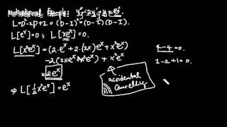
For the equation y'' - y = e^x, the particular solution can be derived through variation of parameters, starting with known solutions from the homogeneous equation.
When modeling forced vibrations in engineering structures, the method of variation of parameters can yield solutions accommodating complex external forcing functions.
Memory Aids
Interactive tools to help you remember key concepts
Rhymes
To find y_p with two u's, plug them in and hear the clues.
Stories
Once upon a time, there were two functions, y1 and y2, who wanted to become a part of a larger solution in a land of equations. They decided to use the magic of parameters to find their way into a bigger family of solutions.
Memory Tools
Remember 'CUPS' for the steps: Construct, Use constraints, Parameterize, Solve.
Acronyms
PES - Parameters, Equations, Solve.
Flash Cards
Glossary
- Variation of Parameters
A method for finding particular solutions of non-homogeneous linear differential equations using known solutions of the corresponding homogeneous equations.
- Homogeneous Equation
A differential equation where the dependent variable and its derivatives appear without any additional terms (such as forcing functions).
- Wronskian
A determinant used in differential equations, particularly in the context of variation of parameters, to establish linear independence of solutions.
- Cramer’s Rule
A mathematical theorem used to solve a system of linear equations using determinants.
- NonHomogeneous Equation
A differential equation that has terms that are not solely dependent on the dependent variable and its derivatives.
Reference links
Supplementary resources to enhance your learning experience.