
Solution by Variation of Parameters
Enroll to start learning
You’ve not yet enrolled in this course. Please enroll for free to listen to audio lessons, classroom podcasts and take practice test.
Interactive Audio Lesson
Listen to a student-teacher conversation explaining the topic in a relatable way.
Introduction to Non-Homogeneous Differential Equations
🔒 Unlock Audio Lesson
Sign up and enroll to listen to this audio lesson

Today, we're discussing non-homogeneous differential equations. Can anyone tell me what a non-homogeneous term means?

I think it's when the equation includes a function that isn't just zero.
Exactly! In our general form, g(x) represents that non-homogeneous term, which can involve various functions. Can someone give me an example of such a function?

Like sin(x) or e^x?
Yes! These are great examples. Remember, non-homogeneous terms can include polynomial, exponential, or trigonometric functions. This leads us to the need for a method to solve these equations when traditional methods, like undetermined coefficients, aren't applicable.

So, that's where variation of parameters comes in?
Exactly! Variation of parameters is a powerful tool for finding a particular solution. Let's dive deeper into how we derive that.
Deriving the Parameters
🔒 Unlock Audio Lesson
Sign up and enroll to listen to this audio lesson

Now, to find a specific solution to our non-homogeneous equation, we assume a form involving unknown functions u_1 and u_2. Can anyone remember the form of that assumption?

I think it was y_p = u_1(x)y_1 + u_2(x)y_2?
That's correct! To simplify our work, we impose a constraint on u_1 and u_2. What do you think that constraint is?
Is it that their derivatives sum to zero?
Right! The constraint states that u_1' y_1 + u_2' y_2 = 0. This makes differentiation manageable. Now, once we differentiate our assumed form, we substitute everything back into our original equation to obtain a system of equations!
So that's how we can isolate u_1 and u_2!
Exactly! This leads us to their derivation using the Wronskian. Let's see how that works next.
Computing the Wronskian
🔒 Unlock Audio Lesson
Sign up and enroll to listen to this audio lesson
Who can explain what the Wronskian is and why it’s important?
Isn’t the Wronskian a determinant that shows whether the functions are linearly independent?
Exactly! For our functions y_1 and y_2, we calculate W(x) = y_1 y_2' - y_2 y_1'. It helps in finding u_1 and u_2 using our derived formulas.
How do we go from the Wronskian to actually finding u_1 and u_2?
Good question! We use the equations: u_1' = -y_2 g(x) / W(x) and u_2' = y_1 g(x) / W(x). After finding these functions, we integrate them to get u_1 and u_2.
And that's our particular solution once we substitute those back!
Exactly! And remember, this method is powerful for any function g(x).
Introduction & Overview
Read summaries of the section's main ideas at different levels of detail.
Quick Overview
Standard
Variation of parameters is introduced as a more general method than undetermined coefficients for obtaining particular solutions to non-homogeneous linear differential equations. The section covers the general form of second-order linear differential equations, the principle behind variation of parameters, and a systematic approach to derive the solution.
Detailed
Solution by Variation of Parameters
Overview
In the context of engineering applications, many systems are modeled using differential equations. Particularly for non-homogeneous linear differential equations, solving for particular solutions can be challenging if using methods like undetermined coefficients. The method of variation of parameters provides a versatile approach to achieve this.
Key Concepts
-
General Form of a Differential Equation: A second-order linear non-homogeneous differential equation can be expressed as
y'' + p(x)y' + q(x)y = g(x). Here, y is the dependent variable, x is the independent variable, and g(x) represents the non-homogeneous term. - Homogeneous Solution: To solve the equation, one must first determine the general solution of the corresponding homogeneous equation.
- Principle of Variation of Parameters: Using two linearly independent solutions of the homogeneous part (y_1 and y_2), we can construct a proposed solution for the non-homogeneous equation by introducing unknown functions u_1 and u_2 such that y_p = u_1(x)y_1 + u_2(x)y_2.
- Deriving Parameters: After differentiating and applying a constraint to simplify the equation, a system of equations is derived, from which u_1 and u_2 can be determined. The Wronskian helps compute these parameters effectively.
- Applications: This technique is crucial in fields such as civil engineering to solve problems related to beam deflections, vibrations, etc.
Summary
The section introduces variation of parameters as a robust tool for finding particular solutions to differential equations, highlighting its advantage over traditional methods, its derivation, examples, common mistakes, and applications in engineering.
Youtube Videos


Audio Book
Dive deep into the subject with an immersive audiobook experience.
Introduction to Variation of Parameters
Chapter 1 of 5
🔒 Unlock Audio Chapter
Sign up and enroll to access the full audio experience
Chapter Content
In many engineering applications, especially in civil engineering, differential equations model real-world systems such as structural deflection, fluid flow, and heat conduction. Often, the equations encountered are non-homogeneous linear differential equations, where the method of undetermined coefficients may not be applicable due to the form of the non-homogeneous term. In such cases, the method of variation of parameters becomes a powerful and general technique to obtain a particular solution.
Detailed Explanation
In engineering, we often need to solve differential equations that describe physical systems. These equations can be complex, especially when they are non-homogeneous, meaning they include a forcing function (or external influence). The traditional method of undetermined coefficients works well for specific types of forcing functions, but when the function doesn't fit these types, we turn to variation of parameters. This method allows us to find a particular solution to a broader range of problems by varying parameters instead of undetermined coefficients.
Examples & Analogies
Think of it like trying to tune a musical instrument. If you only know how to play one specific tune (the method of undetermined coefficients), you might struggle when asked to play different songs (different forcing functions). Variation of parameters is like learning to improvise—you can play along to any song, adjusting your approach as needed.
General Form of a Non-Homogeneous Second-Order Linear Differential Equation
Chapter 2 of 5
🔒 Unlock Audio Chapter
Sign up and enroll to access the full audio experience
Chapter Content
A general second-order linear non-homogeneous differential equation is given by:
y′′+p(x)y′+q(x)y =g(x)
Where:
• y is the dependent variable (typically displacement, temperature, etc.)
• x is the independent variable (time, distance, etc.)
• p(x), q(x): Coefficient functions
• g(x): Non-homogeneous term (external input or forcing function)
The solution to this equation is given by:
y(x)=y_h(x)+y_p(x)
Where:
• y_h(x): General solution to the homogeneous equation y′′+p(x)y′+q(x)y =0
• y_p(x): Particular solution to the non-homogeneous equation.
Detailed Explanation
The presented equation is fundamental to understanding how we solve differential equations in engineering. The equation consists of the second derivative of y, its first derivative, and the function itself, alongside coefficients and an external influence g(x). The total solution y(x) is made up of two parts: the homogeneous solution, which addresses the system without external forces, and the particular solution, which accounts for those external forces. This decomposition helps us solve complex systems by breaking them down into manageable parts.
Examples & Analogies
Imagine you're trying to determine how much a bridge sways (y) under normal conditions (homogeneous) and during a storm with strong winds (non-homogeneous). First, you would calculate how the bridge behaves without the wind (the homogeneous solution). Then, you would add in the effect of the wind (the particular solution) to get a complete picture of the bridge's sway.
Principle of the Variation of Parameters
Chapter 3 of 5
🔒 Unlock Audio Chapter
Sign up and enroll to access the full audio experience
Chapter Content
Suppose we already have the solution to the corresponding homogeneous equation: y′′+p(x)y′+q(x)y =0
Let the two linearly independent solutions of the homogeneous part be y1(x) and y2(x). Then the general solution of the homogeneous equation is:
y_h(x)=C1y1(x)+C2y2(x)
To find a particular solution y_p(x) to the non-homogeneous equation, we assume:
y_p(x)=u_1(x)y_1(x)+u_2(x)y_2(x)
Here, u_1(x) and u_2(x) are functions to be determined.
Detailed Explanation
The principle of variation of parameters hinges on leveraging the known solutions of the homogeneous equation to develop a particular solution. By assuming that the particular solution can be constructed as a linear combination of these solutions, weighted by unknown functions u_1 and u_2, we can derive the particular solution to the non-homogeneous equation. This approach allows us to account for the external influences that change the behavior of the system.
Examples & Analogies
Consider a chef who knows how to make a basic bread recipe. If they want to add unique flavors—like herbs or spices—they can use the original recipe (the homogeneous solution) and replace standard ingredients with new ones (the weighted functions). This way, they create a unique variant of the bread that still maintains the foundational structure.
Derivation of the Variation of Parameters Formula
Chapter 4 of 5
🔒 Unlock Audio Chapter
Sign up and enroll to access the full audio experience
Chapter Content
Differentiate y_p(x):
y_p(x)=u_1(x)y_1(x)+u_2(x)y_2(x)
To simplify the derivation, we impose a constraint:
u_1(x)y_1(x)+u_2(x)y_2(x)=0
Then:
y_p'(x)=u_1'(x)y_1(x)+u_1(x)y_1'(x)+u_2'(x)y_2(x)+u_2(x)y_2'(x)
Differentiate again:
y_p''(x)=u_1'(x)y_1'(x)+u_1(x)y_1''(x)+u_2'(x)y_2'(x)+u_2(x)y_2''(x)
Now substitute into the original non-homogeneous equation: y''+p(x)y'+q(x)y=g(x). After substituting and simplifying using the homogeneous equation, we arrive at a system of equations for u_1 and u_2.
Detailed Explanation
In order to derive the formula for the variation of parameters, we need to differentiate our assumed solution multiple times. The key is imposing a constraint that simplifies the calculations. By ensuring that the linear combination of u_1 and u_2 vanishes, we reduce complexity while solving for these functions. Once we perform substitutions and simplifications, we obtain a manageable system of equations that helps isolate u_1 and u_2, leading us to our particular solution.
Examples & Analogies
Think of this as a detective working to solve a mystery. The detective collects clues (differentiates) from various sources (the initial assumption). To keep the investigation focused, they set certain rules about what types of information to pursue (the constraint). As these clues are analyzed (substituted into the main theory), they help the detective narrow down potential suspects (find u_1 and u_2) until the case is solved.
Step-by-Step Procedure
Chapter 5 of 5
🔒 Unlock Audio Chapter
Sign up and enroll to access the full audio experience
Chapter Content
- Solve the homogeneous equation to find two linearly independent solutions y_1(x), y_2(x).
- Compute the Wronskian W(x)=y_1y_2'-y_1'y_2.
- Compute u_1(x) and u_2(x) using:
u_1(x)=−(y_2g)/(W), u_2(x)=(y_1g)/(W). - Integrate to find u_1(x),u_2(x).
- Construct the particular solution:
y_p(x)=u_1(x)y_1(x)+u_2(x)y_2(x). - Write the general solution as:
y(x)=y_h(x)+y_p(x).
Detailed Explanation
The step-by-step procedure provides a systematic way to approach problems involving non-homogeneous differential equations. In the first step, we find the solutions to the associated homogeneous equation, which serves as a foundation. The Wronskian helps us measure the independence of our chosen solutions. Subsequent steps involve calculating the functions u_1 and u_2, integrating to find their explicit forms, and then using these to build the particular solution. Finally, we combine this with the homogeneous solution to arrive at the complete solution.
Examples & Analogies
Think of following a recipe to bake a cake. You start by mixing the basic ingredients (solving the homogeneous equation). Next, you check that your ingredients are fresh and usable (compute the Wronskian). You then follow specific steps to add flavors and decorations (compute and integrate u_1 and u_2). Finally, you bake the cake (construct the particular solution) and serve it (write the general solution) for everyone to enjoy!
Key Concepts
-
General Form of a Differential Equation: A second-order linear non-homogeneous differential equation can be expressed as
-
y'' + p(x)y' + q(x)y = g(x). Here, y is the dependent variable, x is the independent variable, and g(x) represents the non-homogeneous term.
-
Homogeneous Solution: To solve the equation, one must first determine the general solution of the corresponding homogeneous equation.
-
Principle of Variation of Parameters: Using two linearly independent solutions of the homogeneous part (y_1 and y_2), we can construct a proposed solution for the non-homogeneous equation by introducing unknown functions u_1 and u_2 such that y_p = u_1(x)y_1 + u_2(x)y_2.
-
Deriving Parameters: After differentiating and applying a constraint to simplify the equation, a system of equations is derived, from which u_1 and u_2 can be determined. The Wronskian helps compute these parameters effectively.
-
Applications: This technique is crucial in fields such as civil engineering to solve problems related to beam deflections, vibrations, etc.
-
Summary
-
The section introduces variation of parameters as a robust tool for finding particular solutions to differential equations, highlighting its advantage over traditional methods, its derivation, examples, common mistakes, and applications in engineering.
Examples & Applications
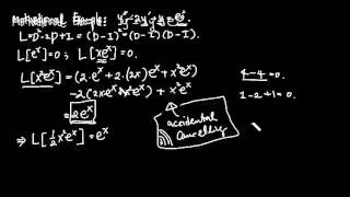
An example is solving y'' + 4y = e^x using variation of parameters.
Another example involves finding particular solutions when g(x) is a polynomial.
Memory Aids
Interactive tools to help you remember key concepts
Rhymes
In equations that are non-homogeneous, variation helps us find the bonus.
Stories
Imagine a builder trying to calculate how a beam will bend under different loads. By applying variation of parameters, they can accurately adjust for the unique situations.
Memory Tools
Think of 'PV= nRT' in chemistry to remember the steps: Parameters Verified - find the Wronskian, then solve for the particular solution.
Acronyms
P=Parameters; V=Verify Wronskian; S=Substitute; S=Solve.
Flash Cards
Glossary
- NonHomogeneous Differential Equation
A differential equation that has a non-zero term, generally expressed as g(x).
- Homogeneous Solution
The solution to the homogeneous part of the differential equation, typically expressed as y_h.
- Wronskian
A determinant used to assess linear independence of solutions.
- Particular Solution
A solution to the non-homogeneous equation, often represented as y_p.
- Variation of Parameters
A method used to find particular solutions of non-homogeneous differential equations.
Reference links
Supplementary resources to enhance your learning experience.