
Long Run Supply Curve of a Firm
Enroll to start learning
You’ve not yet enrolled in this course. Please enroll for free to listen to audio lessons, classroom podcasts and take practice test.
Interactive Audio Lesson
Listen to a student-teacher conversation explaining the topic in a relatable way.
Introduction to Long Run Supply Curve
🔒 Unlock Audio Lesson
Sign up and enroll to listen to this audio lesson

Welcome class! Today, we are discussing the long run supply curve of a firm. Can anyone tell me how long run decisions differ from short-run ones?

In the long run, firms can change all inputs, whereas in the short run only some inputs can be adjusted.
Exactly! In the long run, firms can adjust their production levels entirely based on market conditions. Now, what is the significance of the average cost in determining the supply curve?

The long run supply curve is closely linked to average costs, right? If the market price is below the average cost, firms can't sustain production.
Correct! This also leads us to the concept of the shut down point. Can anyone explain what that is?

It's the point where the price is less than the average cost, meaning firms will stop producing.
Great insight! So firms will exit the market if the price doesn't cover their long run average costs.
To summarize: The long run supply curve reflects how firms react to prices in relation to their average costs, influencing their production decisions.
Profit Maximization in the Long Run
🔒 Unlock Audio Lesson
Sign up and enroll to listen to this audio lesson

Now, let’s discuss profit maximization. What are the critical conditions a firm must meet in the long run?

The price must equal the long run marginal cost, right?
Exactly! That's the first condition. What else?
I think the LRMC must be non-decreasing at the maximum output?
Correct! And the third condition relates to average costs. Can someone explain that?
The price should be greater than or equal to the LRAC to cover total costs.
Well said! Remember, these conditions ensure that firms can sustain themselves and operate efficiently in the long run.
To recap: A profit-maximizing firm must ensure that price equals marginal costs, maintain costs, and cover average costs.
Effects of Price Changes on Supply Curve
🔒 Unlock Audio Lesson
Sign up and enroll to listen to this audio lesson
Let’s talk about how market price changes can influence the supply curve. If the market price increases, what happens to the supply curve?
Firms will want to supply more because they can cover their costs and make profits.
Absolutely! A rightward shift in the supply curve indicates increased output. What can cause a leftward shift then?
If input prices increase, the costs go up, which might decrease the quantity supplied.
Exactly. It’s important for firms to adjust quickly to these changes to remain competitive.
Remember, a firm’s supply curve is sensitive not just to its costs but also to overall market conditions.
To summarize: Price increases lead to more output, while rising costs can reduce output, shifting the supply curve.
Introduction & Overview
Read summaries of the section's main ideas at different levels of detail.
Quick Overview
Standard
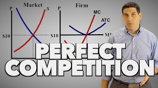
In this section, we delve into the concept of the long run supply curve of a firm within a perfectly competitive market. We analyze the relationship between market price and average costs, explaining the conditions under which firms maximize profits and how these factors influence the firm's supply curve. We also differentiate between short run and long run supply decisions.
Detailed
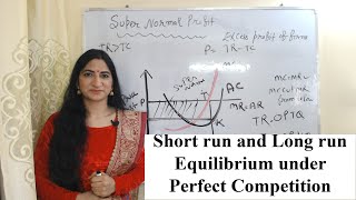
Long Run Supply Curve of a Firm
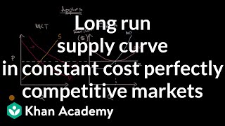
In a perfectly competitive market, the long run supply curve of a firm is crucial for understanding how firms adjust production over time in response to market prices. The long run differs from the short run primarily because firms can adjust all factors of production.
Key Points:
- Price and LRAC Relationship: The long run supply curve is derived from the relationship between market price and long run average cost (LRAC). When the market price exceeds the minimum LRAC, firms will supply positive output. Conversely, if the price falls below this threshold, firms will cease production.
- Profit Maximization Conditions: For a firm to maximize profits in the long run, three conditions must be met:
- Price (P) must equal Long Run Marginal Cost (LRMC).
- LRMC should be non-decreasing at the profit-maximizing output level.
- Price should be greater than or equal to LRAC to cover total costs.
- Supply Decision Considerations: If a firm’s production costs rise or fall due to changes in technology or input prices, its supply curve will shift accordingly. A leftward shift indicates fewer outputs supplied at the same prices, while a rightward shift means more outputs can be supplied.
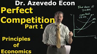
- Shut Down Point: The long run shut down point for a firm occurs at the minimum LRAC, where firms do not cover their costs and will exit the market if the price remains below this point.
Understanding these elements is essential as they shape the behavior of firms in the market and influence overall market supply dynamics.
Youtube Videos


Audio Book
Dive deep into the subject with an immersive audiobook experience.
Deriving the Long Run Supply Curve
Chapter 1 of 4
🔒 Unlock Audio Chapter
Sign up and enroll to access the full audio experience
Chapter Content
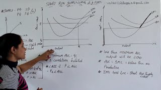
Let us turn to Figure 4.9 and derive the firm’s long run supply curve. As in the short run case, we split the derivation into two parts. We first determine the firm’s profit-maximising output level when the market price is greater than or equal to the minimum (long run) AC. This done, we determine the firm’s profit-maximising output level when the market price is less than the minimum (long run) AC.
Detailed Explanation
In this chunk, we begin the process of deriving the long run supply curve for a firm. This involves dividing the process into two cases based on the market price relative to the firm's average cost. First, we look at situations where the price is at least equal to the minimum average cost (AC), which allows the firm to cover its production costs and earn normal profits. When the price is above this threshold, the firm is incentivized to maximize its output. In the second case, we consider what happens when the market price falls below the minimum average cost, indicating that the firm cannot cover its expenses and consequently would not choose to produce at all in the long run.
Examples & Analogies
Think of a bakery that requires a minimum oven cost to bake bread. If the price of bread rises above the cost of baking (like a market price above its minimum average cost), the bakery will bake as much bread as possible to maximize profits. Conversely, if the price falls below their baking costs, they would shut down their operations to avoid losing money.
Case 1: Price Greater than or Equal to Minimum LRAC
Chapter 2 of 4
🔒 Unlock Audio Chapter
Sign up and enroll to access the full audio experience
Chapter Content
Case 1: Price greater than or equal to the minimum LRAC. Suppose the market price is p1, which exceeds the minimum LRAC. Upon equating p1 with LRMC on the rising part of the LRMC curve, we obtain output level q1. Note also that the LRAC at q1 does not exceed the market price, p1. Thus, all three conditions highlighted in section 3 are satisfied at q1. Hence, when the market price is p1, the firm’s supplies in the long run become an output equal to q1.
Detailed Explanation
In this section of the analysis, when the market price is above the minimum long run average cost (LRAC), it assures the firm that they can not only cover their production costs but also earn profits. Thus, the firm identifies its profit-maximizing output level by finding the point where the long-run marginal cost (LRMC) equals the price. This enables them to set production at levels that maximize potential profits while still staying within the bounds of covering costs; therefore, they produce the quantity q1 as long as the market price remains at p1 or higher.
Examples & Analogies
Imagine a farmer who grows tomatoes. When the market price of tomatoes rises above the cost of water, seeds, and labor, the farmer will plant as many tomatoes as possible to earn profits. If the price continues to rise, the farmer will keep increasing production until the cost of that last bushel of tomatoes equals the market price. This maximizes their profits without risking losses due to high operating costs.
Case 2: Price Less than the Minimum LRAC
Chapter 3 of 4
🔒 Unlock Audio Chapter
Sign up and enroll to access the full audio experience
Chapter Content
Case 2: Price less than the minimum LRAC. Suppose the market price is p2, which is less than the minimum LRAC. We have argued that if a profit-maximising firm produces a positive output in the long run, the market price, p2, must be greater than or equal to the LRAC at that output level. But notice from Figure 4.9 that for all positive output levels, LRAC strictly exceeds p2. In other words, it cannot be the case that the firm supplies a positive output. So, when the market price is p2, the firm produces zero output.
Detailed Explanation
In this scenario, when the market price drops below the minimum average cost, the firm realizes it cannot sustain operations and cover its costs. If producing something would incur greater costs than the revenue generated, the firm opts to cease production altogether in the long run to minimize losses. Hence, their output becomes zero at this price level, as producing no output is financially more feasible than producing at a loss.
Examples & Analogies
Consider a small coffee shop. If the cost of coffee beans, milk, and other supplies exceeds what customers are willing to pay for coffee, the owner would rather close the shop than keep operating at a loss. They might wait for market prices to improve to ensure that when they open again, they can cover their costs and be profitable.
Conclusion on Long Run Supply Curve
Chapter 4 of 4
🔒 Unlock Audio Chapter
Sign up and enroll to access the full audio experience
Chapter Content
Combining cases 1 and 2, we reach an important conclusion. A firm’s long run supply curve is the rising part of the LRMC curve from and above the minimum LRAC together with zero output for all prices less than the minimum LRAC. In Figure 4.10, the bold line represents the long run supply curve of the firm.
Detailed Explanation
The overall conclusion for the long run supply curve illustrates that it consists of two segments: one where the firm will actively supply goods when prices cover production costs and allow for profits, and another where the firm will not produce at all due to insufficient market prices. Therefore, the long run supply curve reflects the range of prices at which firms are willing to produce over the long term, effectively illustrating their responsiveness to market conditions.
Examples & Analogies
Think of a new technology company that produces smartphones. If the price of smartphones exceeds the cost of production, the company will ramp up its manufacturing. Conversely, if a major competitor drops prices substantially, leading to prices below production costs, the tech company may halt all production until they can return to a profitable range. This behavior shapes the company's long run supply curve in the technology market.
Key Concepts
-
Long Run Advantages: Firms can adjust all production inputs.
-
Price and Average Cost: The relationship determines supply levels.
-
Profit Maximization: Requires equal marginal cost and market price.
-
Shut Down Point: Defines the minimum acceptable price for production.
Examples & Applications
If a firm sees that the market price of their product exceeds their average cost, they will increase production to maximize profits.
When the input costs rise, a firm may reduce the quantity supplied or increase prices to maintain profitability.
Memory Aids
Interactive tools to help you remember key concepts
Rhymes
Cost low, produce more, keep the profit in store.
Stories
Imagine a farmer who grows apples. When the apple price rises, he plants more trees, maximizing his harvest. If he can't cover his costs, he won't plant at all, reflecting the shut down point.
Memory Tools
To remember profit maximization conditions: P = MC, MC up, price covers AC: PMU (Price - Marginal Cost, Marginal Cost rise, Price covers Average Cost).
Acronyms
LRAC - Long Run Average Cost represents total output divided by the total input over long term.
Flash Cards
Glossary
- Long Run Supply Curve
The curve that shows the quantity of goods firms are willing to supply at different prices in the long run, where all inputs can be varied.
- Average Cost (AC)
Total cost divided by the number of goods produced; a measure of the per-unit cost of production.
- Marginal Cost (MC)
The additional cost incurred from producing one more unit of a good.
- Shut Down Point
The price level at which a firm's revenue just covers its variable costs, below which the firm will cease production.
- Profit Maximization
The process by which a firm determines the price and output level that leads to the highest possible level of profit.
Reference links
Supplementary resources to enhance your learning experience.